Time Traveler

안녕하세요.

이번 글에서는 CNN 모델의 학습할 방향성을 정해주기 위한 loss function, opimizer, learning rate policy를 설정해주는 코드들을 살펴보도록 하겠습니다.

import torch.nn as nn
import torch.optim as optim
from torch.optim import lr_scheduler

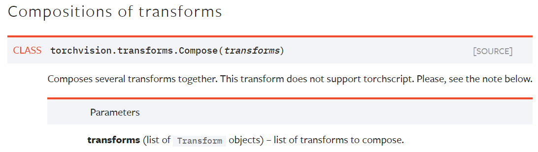
1. Loss function 설정

torch.nn 을 살펴보면 다양한 neural network를 제공해주는 것 외에 loss function도 제공해주고 있다는 걸 확인할 수 있습니다.

https://pytorch.org/docs/stable/nn.html

CNN 학습을 위해 torch.nn에서 제공해주는 CrossEntropyLoss를 사용합니다. (다른 loss function도 사용가능 하지만 보통은 crossentropy loss를 사용합니다)

2. optimizer 정의 (Feat. 최신 optimizer 사용방식)

torch.optim 이라는 패키지를 살펴보면 다양한 optimizer를 제공해준다는 것을 알 수 있습니다.

(경험상 optimizer를 무엇으로 사용했는지에 따라 딥러닝 모델 성능에 많은 영향을 끼치는걸 확인할 수 있었기 때문에 어떠한 optimizer를 사용할지 잘 결정하는 것이 중요합니다.)

https://pytorch.org/docs/stable/optim.html

(↓↓↓optimizer 관련 내용 정리한 글↓↓↓)

https://89douner.tistory.com/46

torch.optim은 가장 기본이 되는 optimizer들을 제공합니다.

하지만 최신 SOTA 성능의 optimizer들은 제공하지 않는 경우가 많죠.

그래서 SOTA 성능의 optimizer를 이용하기 위해서는 다른 방법을 찾아야 합니다.

보통 SOTA optimizer 같은 경우는 논문으로 출판할 때, 해당 optimizer를 이용할 수 있게 github에 업로드합니다. 업로드된 optimizer를 패키지로 다운받아 pytorch, tensorflow와 연동해서 사용하면 됩니다.

예를 들어, adabelief optimizer라는 최신 optimizer가 나왔다고 하면 아래와 같은 순서를 따라 이용하면 됩니다.

1) adabelief optimizer github 사이트 검색

https://github.com/juntang-zhuang/Adabelief-Optimizer

 2) 위의 사이트에서 언급한대로 adabelief optimizer 패키지 설치

• 여기에서는 pytorch 버전 설치
• 다른 가상환경을 사용하고 있으면 해당 가상환경에 설치하는데 필요한 명령어로 바꾸어 설치 (ex: anaconda)

pip install adabelief-pytorch==0.2.0

 3) 설치한 adabelief optimizer 패키지 설치 후, 해당 optimizer 이용

from adabelief_pytorch import AdaBelief
optimizer_ft = AdaBelief(model.parameters(), lr=1e-3, eps=1e-16, betas=(0.9,0.999), weight_decouple = True, rectify = False)

3. learning rate scheduler (policy) 정의

앞서 optimizer를 정의 했다면, learning rate policy를 정해주어야 합니다.

기본적인 learning rate policy 역시 torch.opim에서 제공해주니 아래 API를 참고하시면 다양한 learning rate policty를 확인하실 수 있습니다.

https://pytorch.org/docs/stable/optim.html

Learning rate policy는 정말 다양하게 있는데 대표적인 경우들에 대해서 소개하도록 하겠습니다.

1) Step policy

학습을 하다보면 loss가 정체되어 있는 경우가 있습니다. 이 경우 early stoping을 하여 학습을 종료시키는 경우도 있지만 아래 "그림10"에서 처럼 정체되는 순간 learning rate을 감소시켜주면 loss가 다시 줄어드는경우도 있습니다. 

이와 같이 계단 형식으로 learning rate을 감소(decay) 시켜주는 learning rate policy 방식을 step decay라고 합니다.

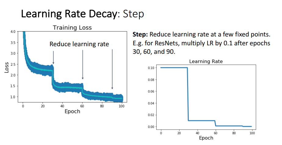
Step decay 방식을 이요하려면 아래와 같이 코드를 작성해주면 됩니다.

아래와 같은 코드를 작성해주면 3번의 epoch 마다 learning rate가 0.1씩 감소하게 됩니다. 

(↓↓↓pytorch에서 제공해주는 step learning rate policy API↓↓↓)

https://pytorch.org/docs/stable/generated/torch.optim.lr_scheduler.StepLR.html#torch.optim.lr_scheduler.StepLR

2) Cosine annealing policy

Pytorch에서는 step learning rate policy외에 cosine annealing policy라는 방식도 제공해줍니다. 

보통은 cosine annealing policy를 warm_up과 같이 사용하는데, 이에 대해서는 뒷 부분에서 설명하도록 하겠습니다.

• optimizer – Wrapped optimizer.
• T_max (int)  – Maximum number of iterations.
• eta_min (float)  – Minimum learning rate. Default: 0.
• last_epoch (int) – The index of last epoch. Default: -1.

(↓↓↓pytorch에서 제공해주는 Cosine Annealing learning rate policy API↓↓↓)

https://pytorch.org/docs/stable/generated/torch.optim.lr_scheduler.CosineAnnealingLR.html#torch.optim.lr_scheduler.CosineAnnealingLR

3) Warm_up policy

초기에는 layer 값들이 굉장히 불안정하기 때문에 너무 큰 learning rate을 적용하면 loss값이 지나치게 커질 수 있습니다. 그래서 초기의 unstable 상태를 고려해 초기 특정 epoch 까지는 learning rate을 천천히 증가시켜주는 방식이 warm_up 방식입니다.

Warm_up을 통해 특정 epoch 까지 learning rate을 증가시키면, 특정 epoch 이후에는 기존 learning rate policy를 적용시켜주어야 합니다. 

아래 그림을 보면 초기 5 epoch 까지는 learning rate을 점진적으로 증가시키고, 5 epoch 이후에는 step policy 또는 cosine annealing policy  확인할 수 있습니다.

Warm_up policy는 pytorch에서 기본 learning rate policy로 제공해주고 있지 않기 때문에 따로 warm_up laerning rate policy 패키지를 설치해야합니다.

3-1) Warm_up policy with step learning rate policy

3-1-1) warm_up step learning rate과 관련된 사이트 검색 

https://github.com/ildoonet/pytorch-gradual-warmup-lr

3-1-2) 패키지 설치

pip install git+https://github.com/ildoonet/pytorch-gradual-warmup-lr.git

3-1-3) 설치된 패키지 이용

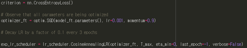
criterion = nn.CrossEntropyLoss()

# Observe that all parameters are being optimized
optimizer_ft = optim.SGD(model_ft.parameters(), lr=0.001, momentum=0.9) 

# Decay LR by a factor of 0.1 every 3 epochs
exp_lr_scheduler = lr_scheduler.StepLR(optimizer_ft, step_size=3, gamma=0.1)
exp_lr_scheduler = GradualWarmupScheduler(optimizer_ft, multiplier=1, total_epoch=5, after_scheduler=exp_lr_scheduler)

3-2) Warm_up policy with cosine annealing learning rate policy

3-2-1) warm_up consine annealing learning rate과 관련된 사이트 검색 

https://github.com/katsura-jp/pytorch-cosine-annealing-with-warmup

3-2-2) 패키지 설치

pip install 'git+https://github.com/katsura-jp/pytorch-cosine-annealing-with-warmup'

3-2-3) 설치된 패키지 이용

from cosine_annealing_warmup import CosineAnnealingWarmupRestarts

criterion = nn.CrossEntropyLoss()
optimizer_ft = optim.SGD(model.parameters(), lr=0.1, momentum=0.9, weight_decay=1e-5) # lr is min lr
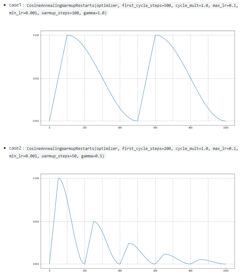
scheduler = CosineAnnealingWarmupRestarts(optimizer, first_cycle_steps=200, cycle_mult=1.0, max_lr=0.1, min_lr=0.001, warmup_steps=50, gamma=1.0)

Cosine annealing with warm_up 과 관련된 hyper parameter들은 아래 그림을 보면 이해하시기 편하실 겁니다. (참고로 gamma부분은 다음 cycle에서 max_lr을 어느 정도 줄여줄지를 결정해주는 hyper parameter 입니다)

Warm_up을 적용시킬 때 batch size에 따라 initial learning rate(=마지막 warm up 단계에서의 learning rate)를 어떻게 설정해 줄 지 결정해 주기도 합니다. 이 부분은 아래 글에서 learning rate warmup 부분을 참고해주시면 될 것 같습니다.

https://89douner.tistory.com/248

4. 요약

지금까지 배운 내용을 잠시 정리 해보겠습니다.

# License: BSD
# Author: Sasank Chilamkurthy

from __future__ import print_function, division

import torch
import torch.nn as nn
import torch.optim as optim
from torch.optim import lr_scheduler
import numpy as np
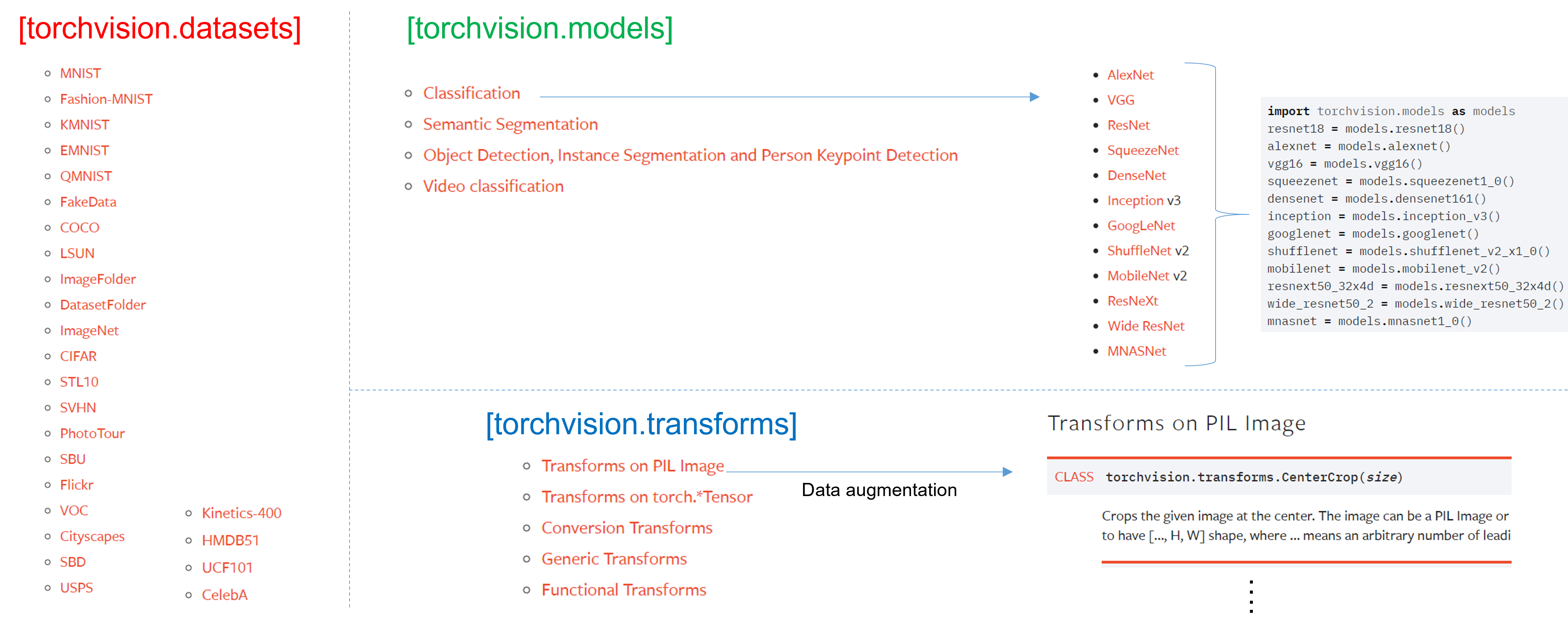
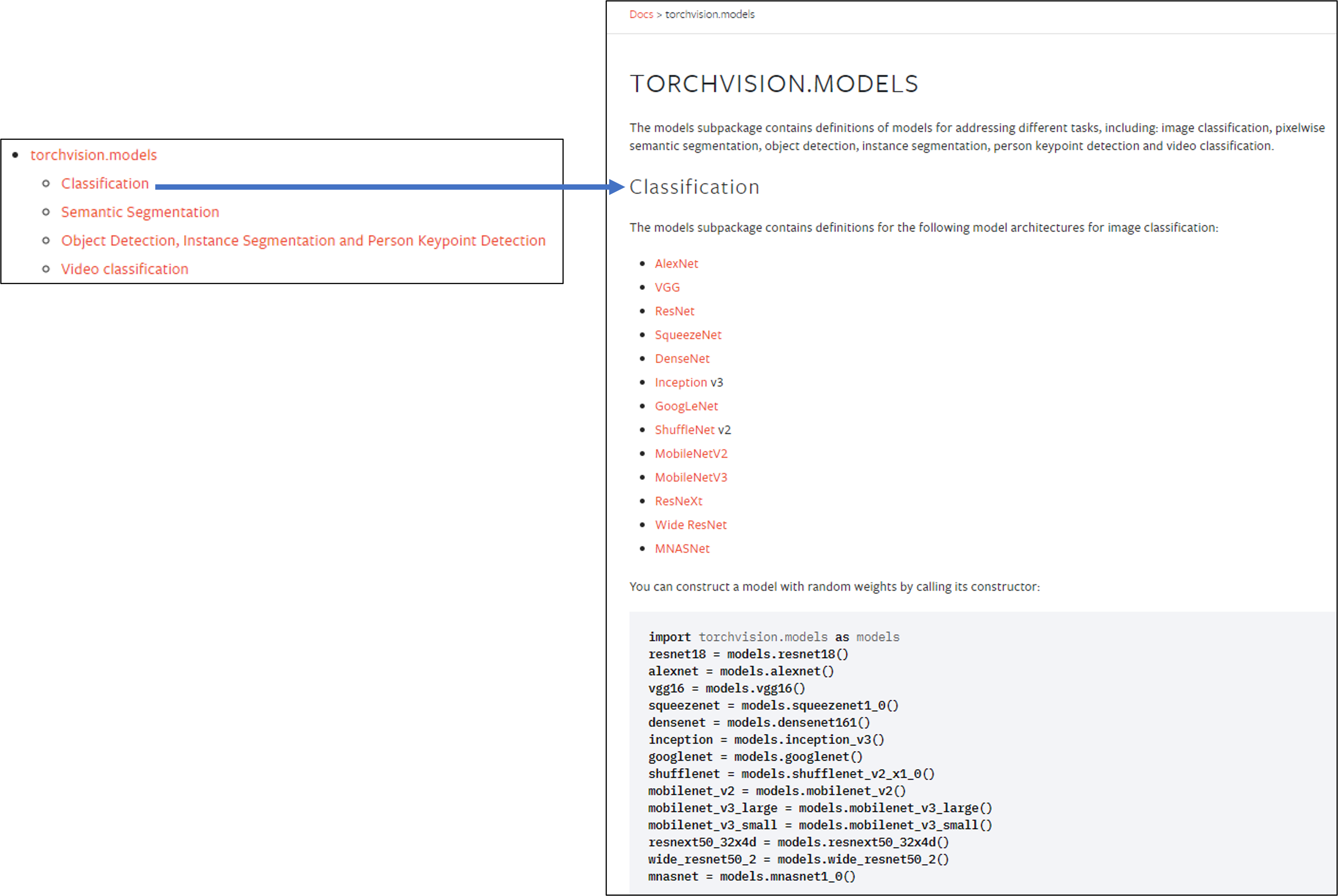
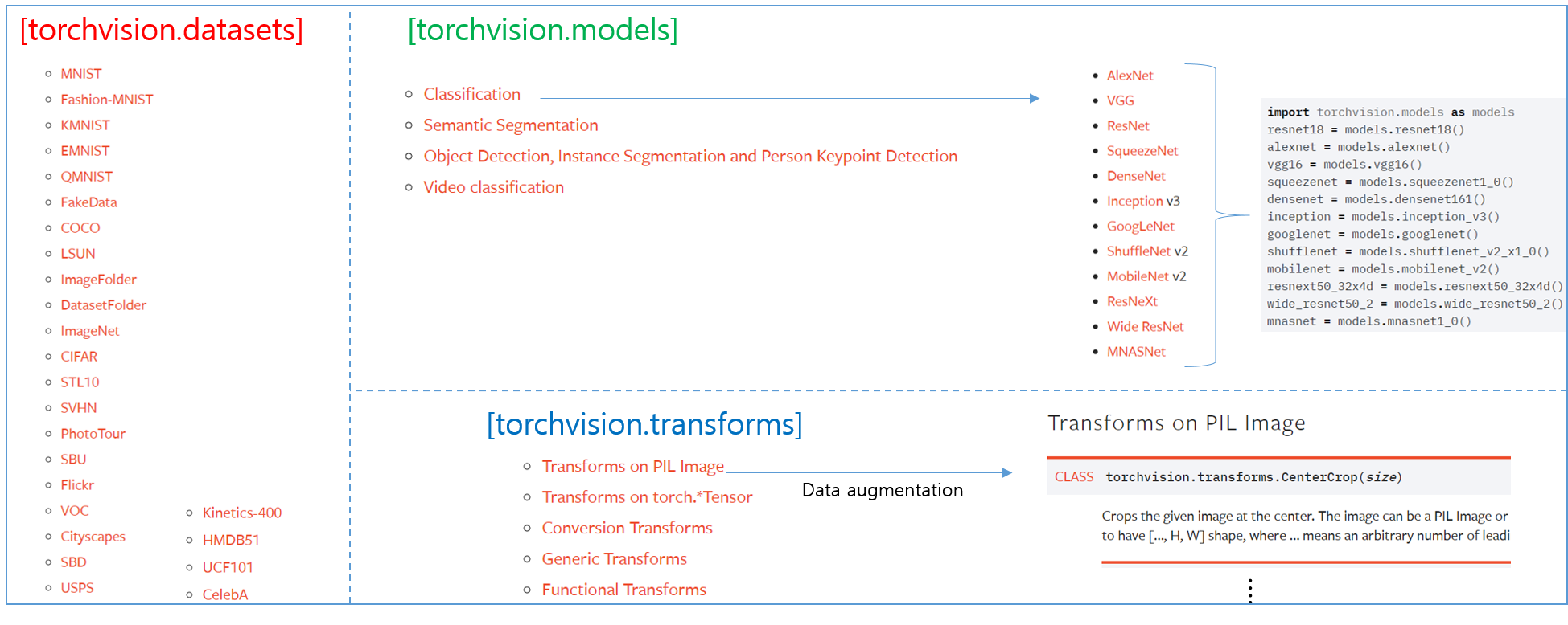
import torchvision
from torchvision import datasets, models, transforms
import matplotlib.pyplot as plt
import time
import os
import copy

plt.ion()   # interactive mode

4-1. Data Load

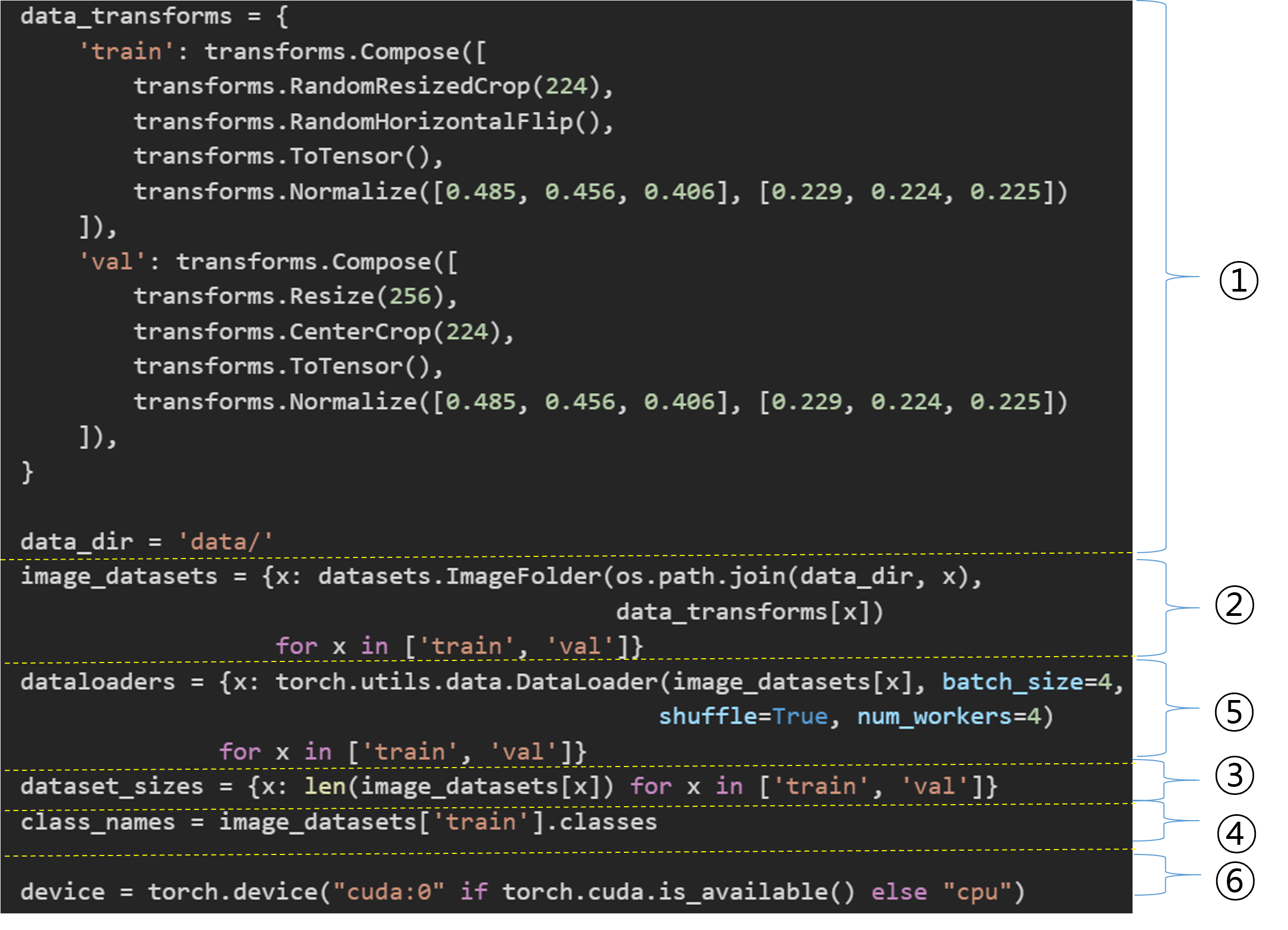
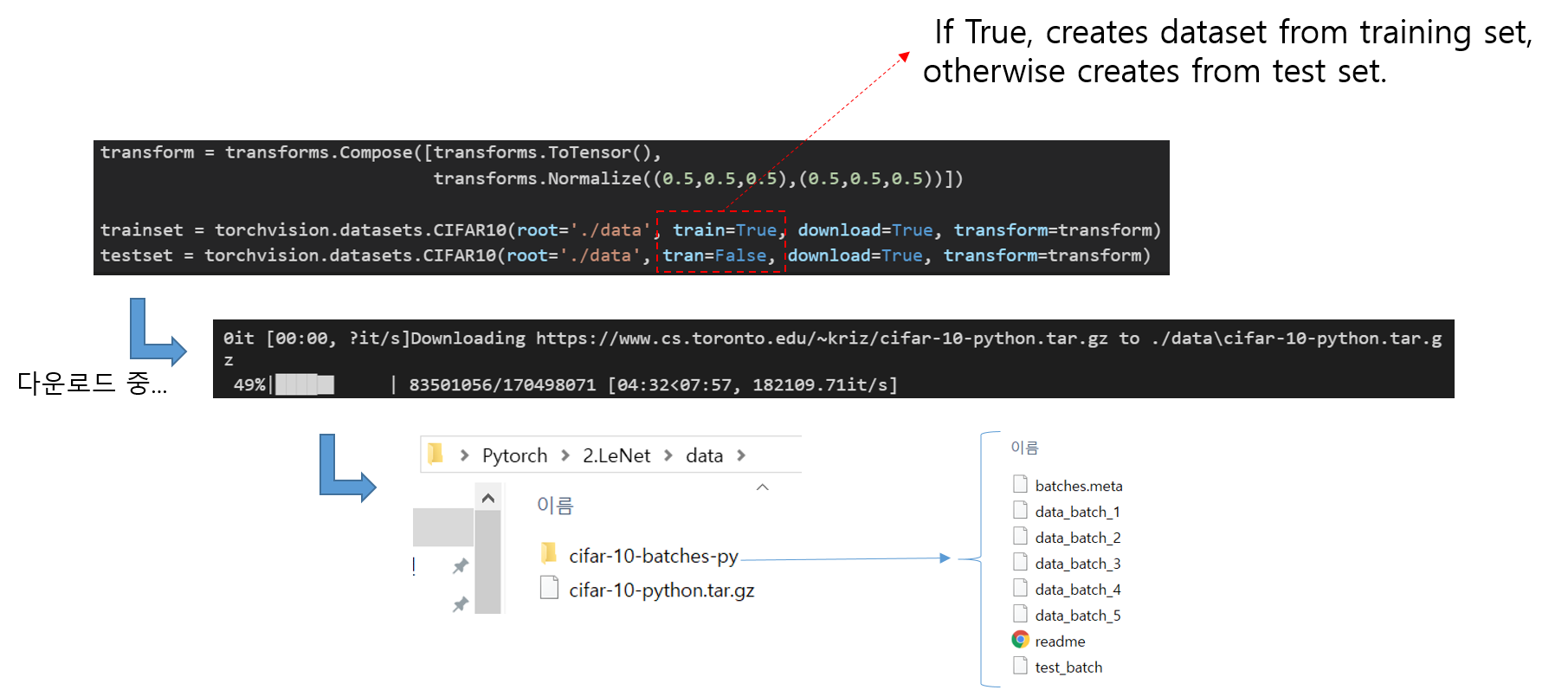
먼저 아래 글을 통해 CNN 학습을 위하 이미지 데이터들을 어떻게 load 하는지에 대해서 설명했습니다.

https://89douner.tistory.com/287?category=994842 

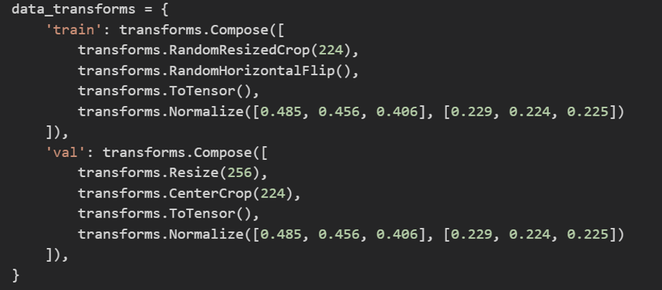
# Data augmentation and normalization for training
# Just normalization for validation
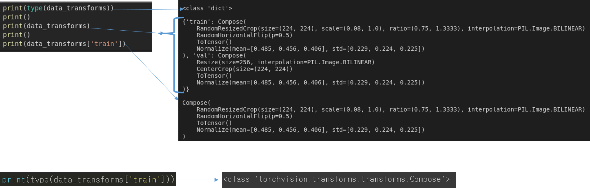
data_transforms = {
    'train': transforms.Compose([
        transforms.RandomResizedCrop(224),
        transforms.RandomHorizontalFlip(),
        transforms.ToTensor(),
        transforms.Normalize([0.485, 0.456, 0.406], [0.229, 0.224, 0.225])
    ]),
    'val': transforms.Compose([
        transforms.Resize(256),
        transforms.CenterCrop(224),
        transforms.ToTensor(),
        transforms.Normalize([0.485, 0.456, 0.406], [0.229, 0.224, 0.225])
    ]),
}

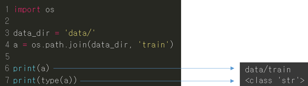
data_dir = 'data/hymenoptera_data'
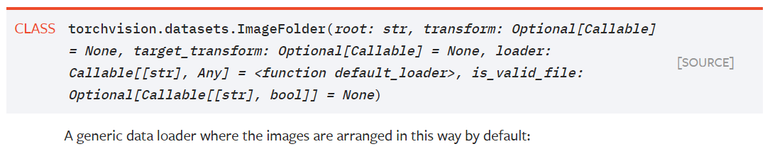
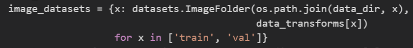
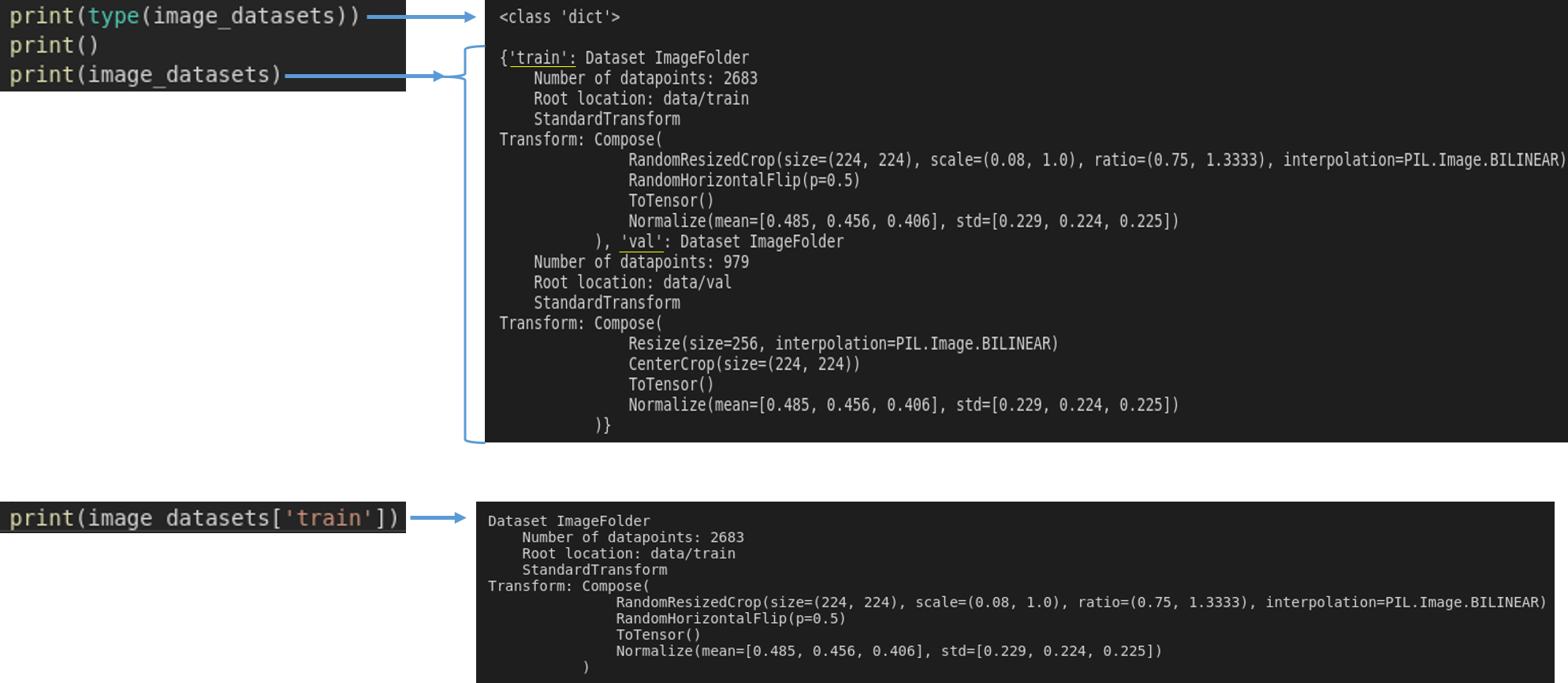
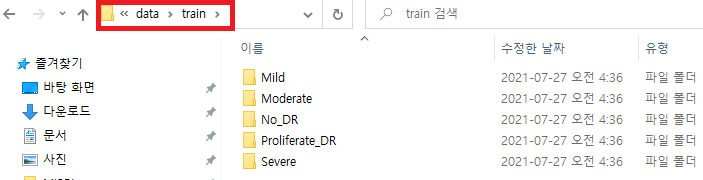
image_datasets = {x: datasets.ImageFolder(os.path.join(data_dir, x),
                                          data_transforms[x])
                  for x in ['train', 'val']}
dataloaders = {x: torch.utils.data.DataLoader(image_datasets[x], batch_size=4,
                                             shuffle=True, num_workers=4)
              for x in ['train', 'val']}
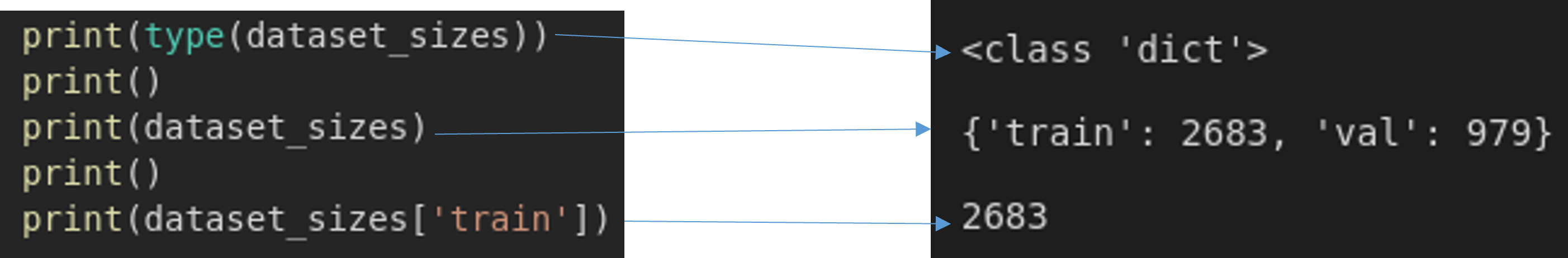
dataset_sizes = {x: len(image_datasets[x]) for x in ['train', 'val']}
class_names = image_datasets['train'].classes

device = torch.device("cuda:0" if torch.cuda.is_available() else "cpu")

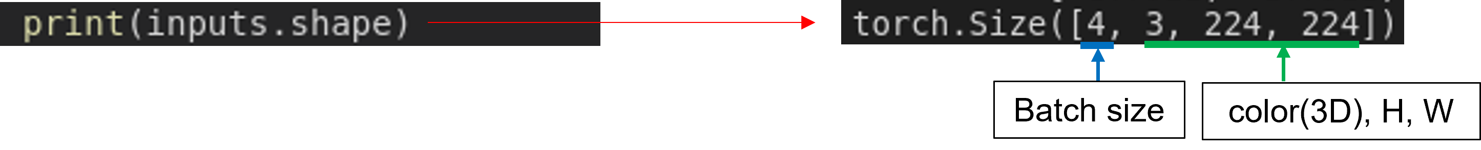
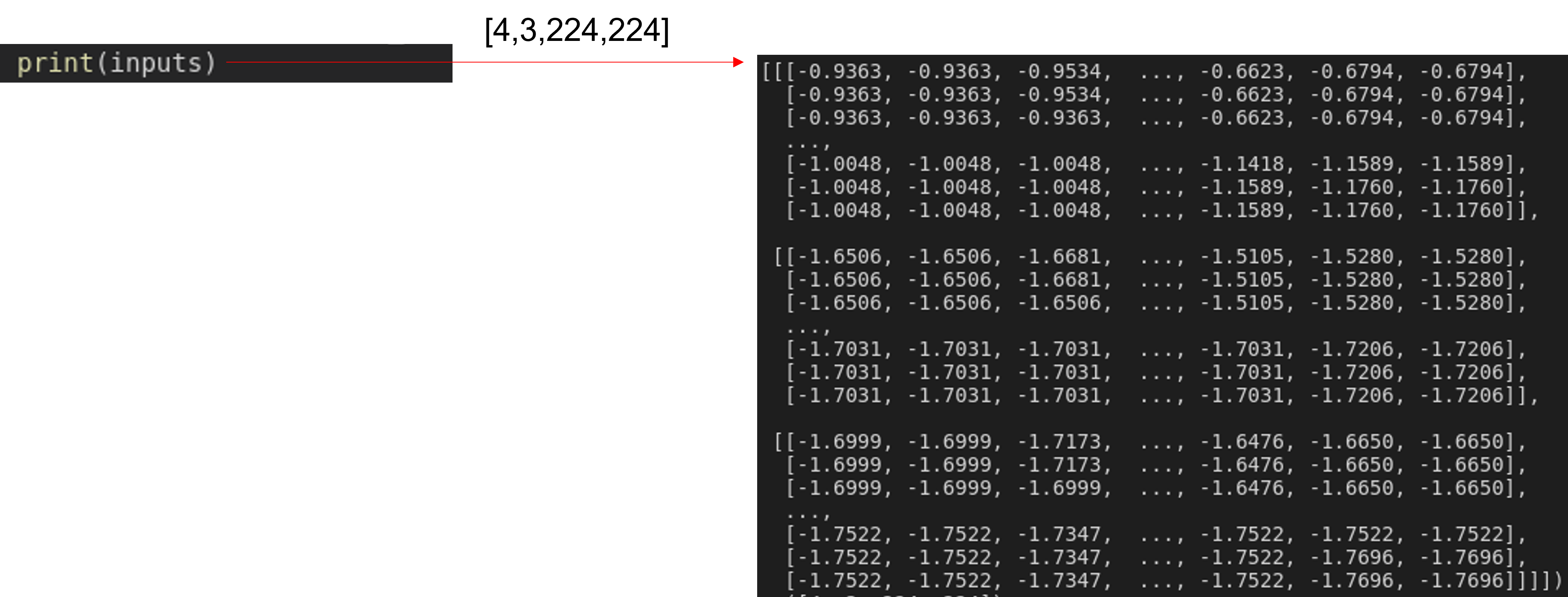
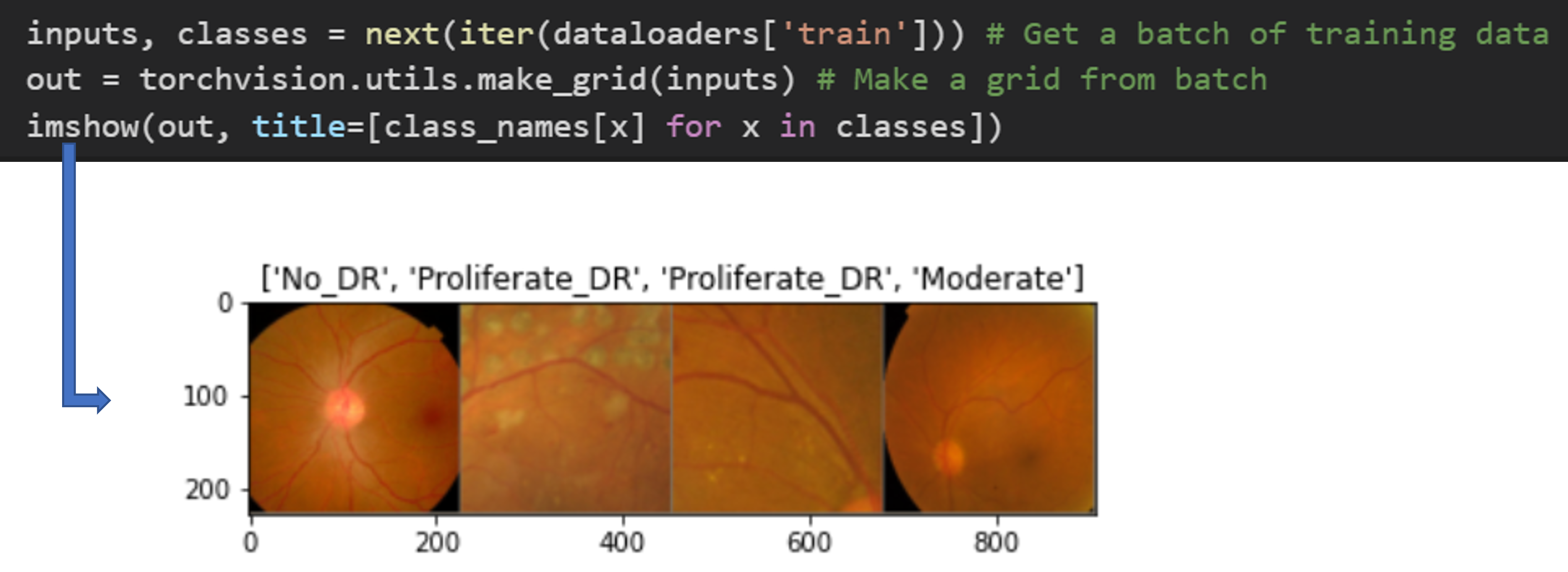
추가적으로 batch 단위로 augmentation이 적용된 이미지 데이터들을 아래 함수로 확인해볼 수 있었습니다.

def imshow(inp, title=None):
    """Imshow for Tensor."""
    inp = inp.numpy().transpose((1, 2, 0))
    mean = np.array([0.485, 0.456, 0.406])
    std = np.array([0.229, 0.224, 0.225])
    inp = std * inp + mean
    inp = np.clip(inp, 0, 1)
    plt.imshow(inp)
    if title is not None:
        plt.title(title)
    plt.pause(0.001)  # pause a bit so that plots are updated


# Get a batch of training data
inputs, classes = next(iter(dataloaders['train']))

# Make a grid from batch
out = torchvision.utils.make_grid(inputs)

imshow(out, title=[class_names[x] for x in classes])

4-2. Data Preprocessing

아래 글을 통해 학습 데이터를 전처리하기 위한 다양한 방식들에 대해서 다루어 봤습니다.

(작성중....)

4-3.  CNN

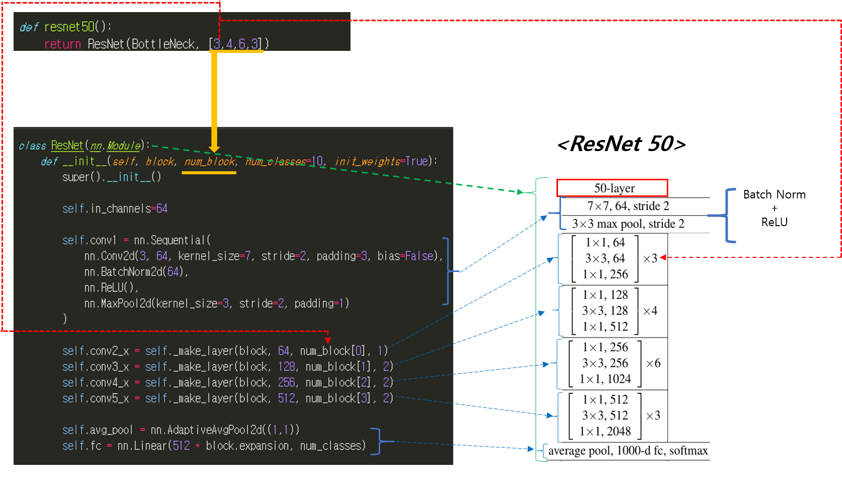
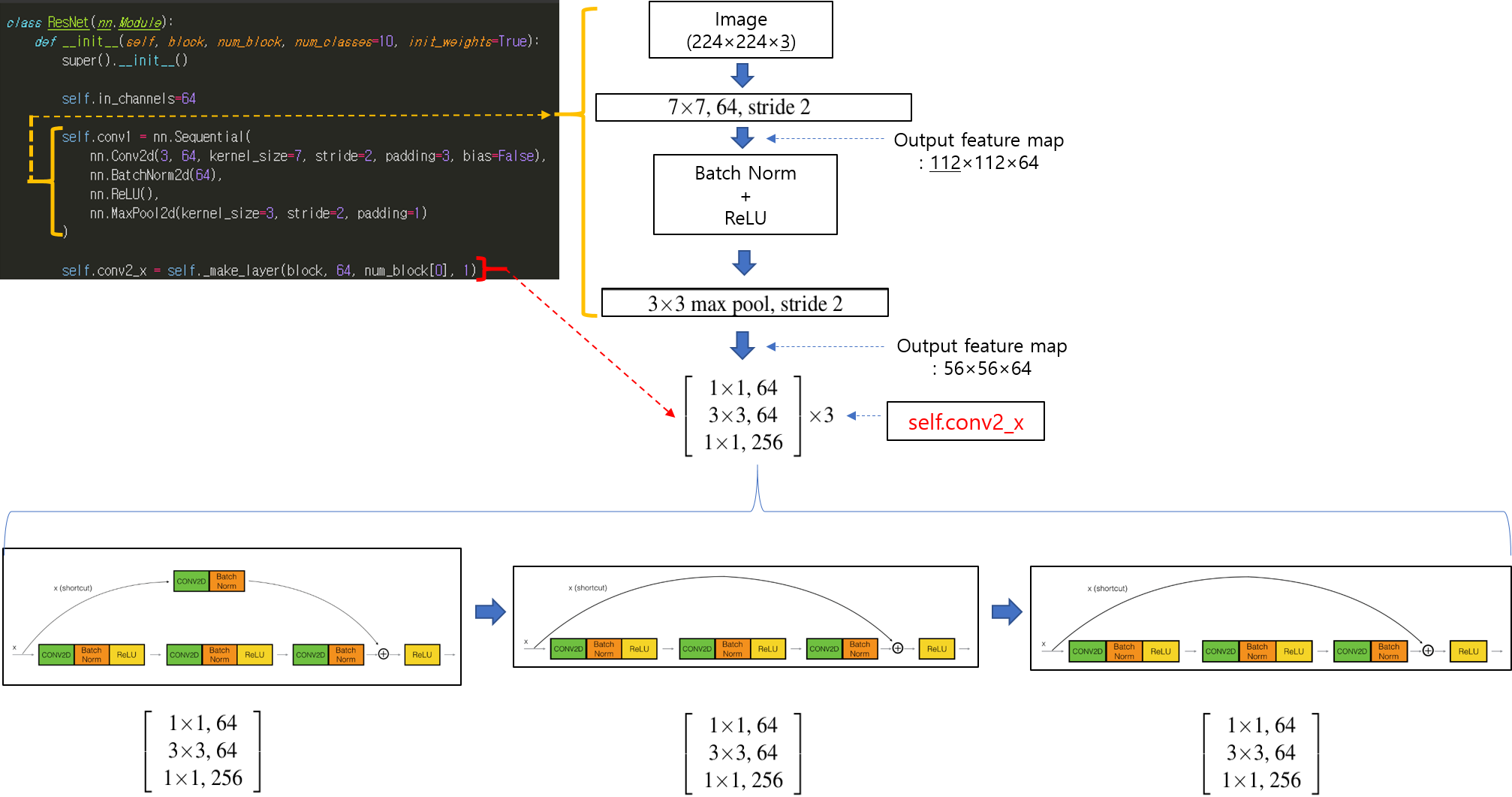
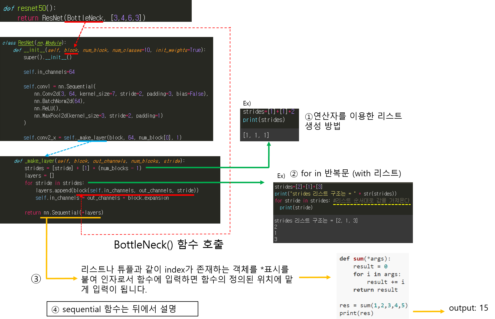
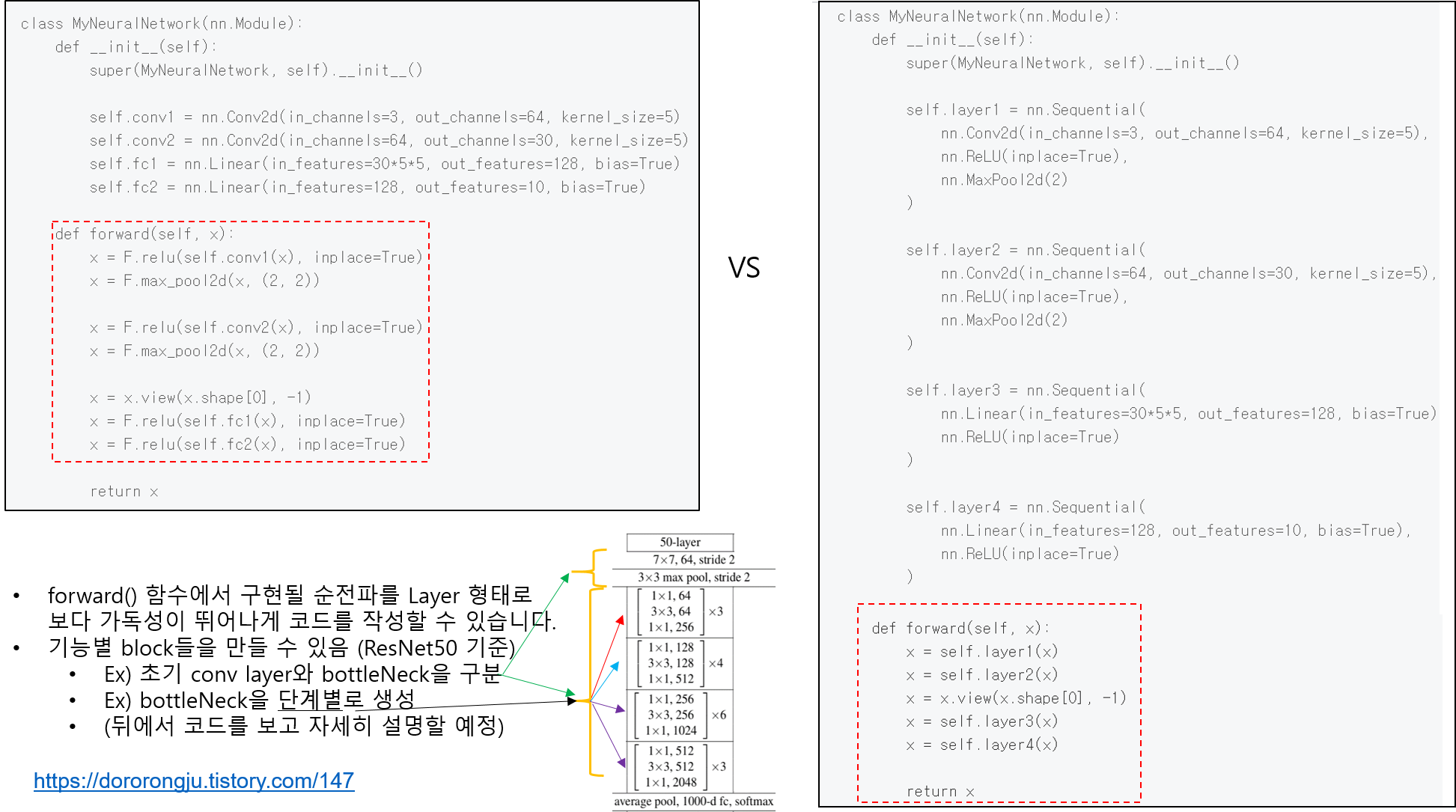
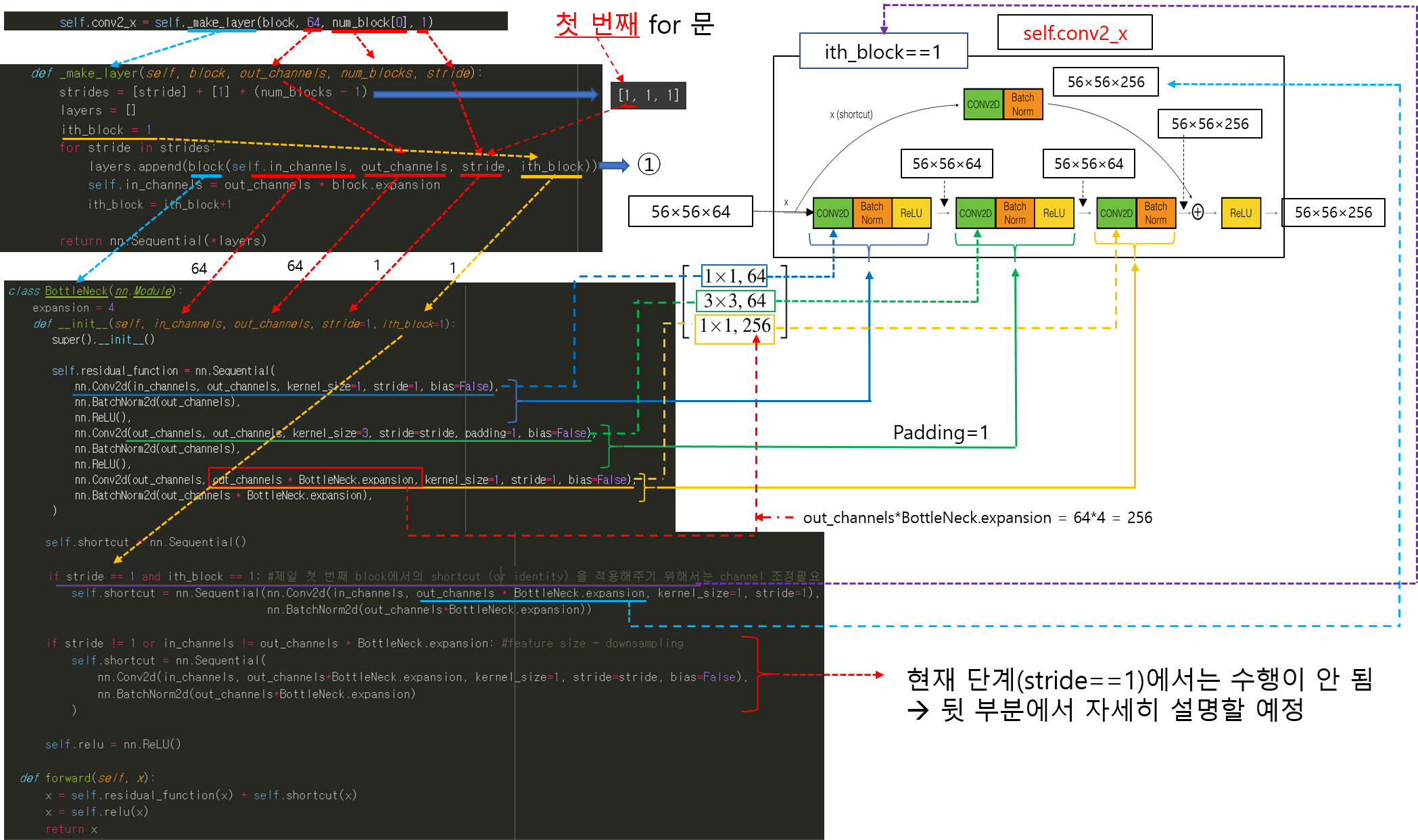
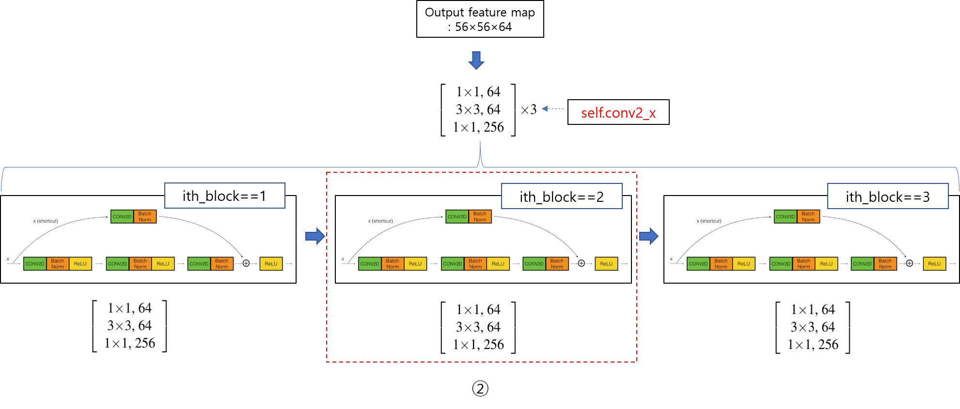
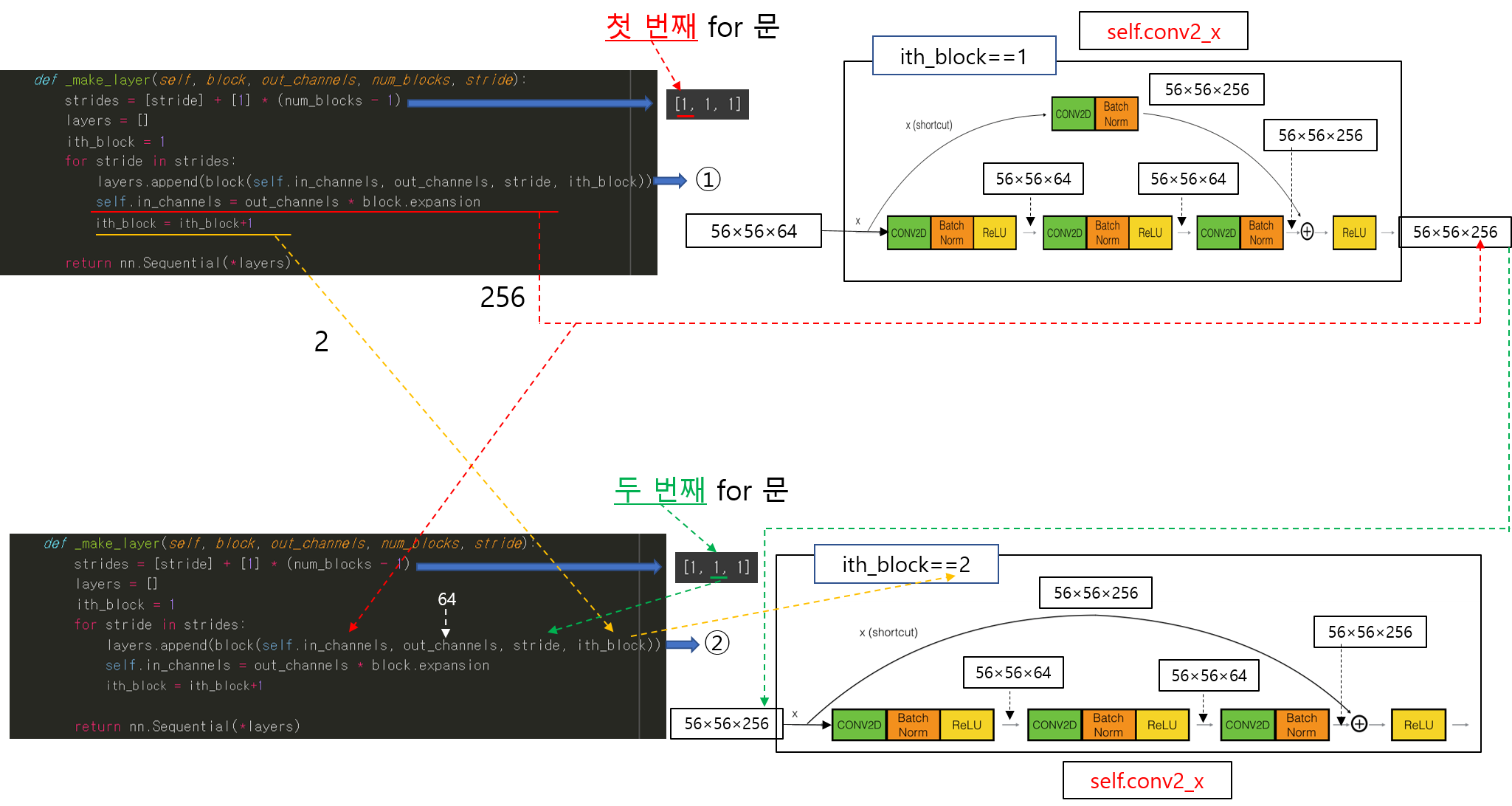
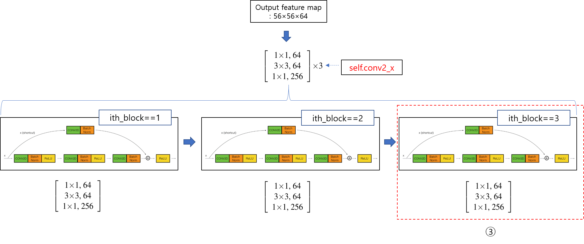
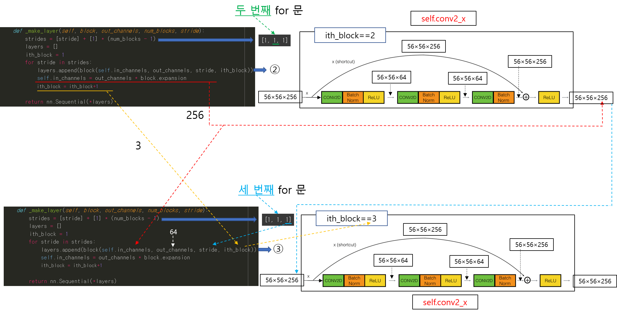
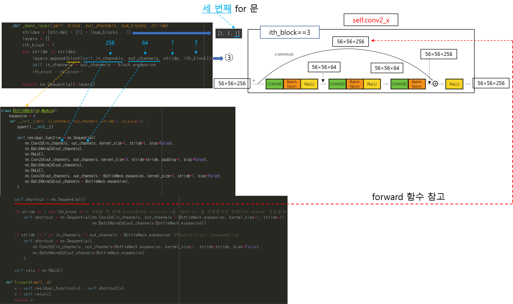
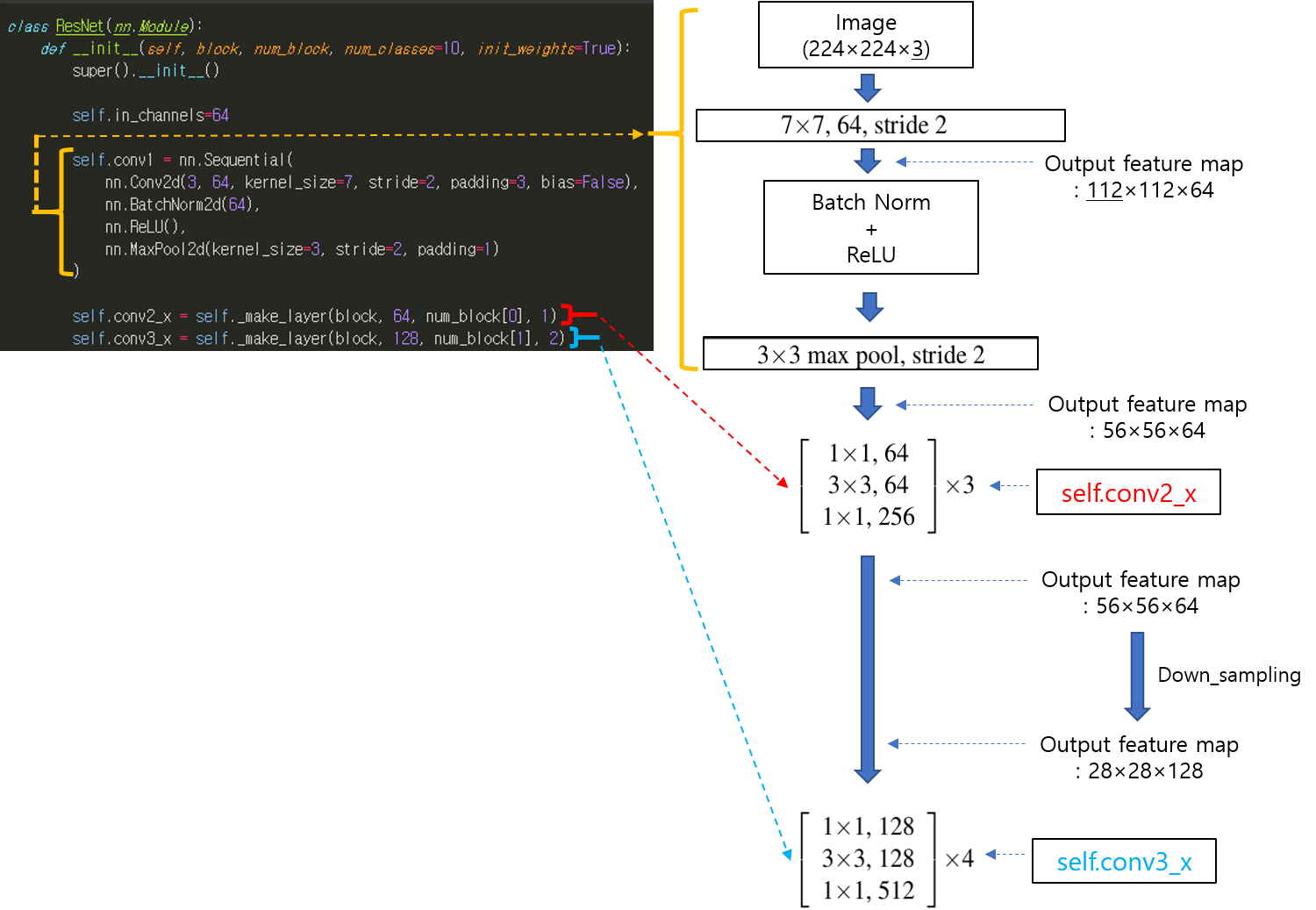
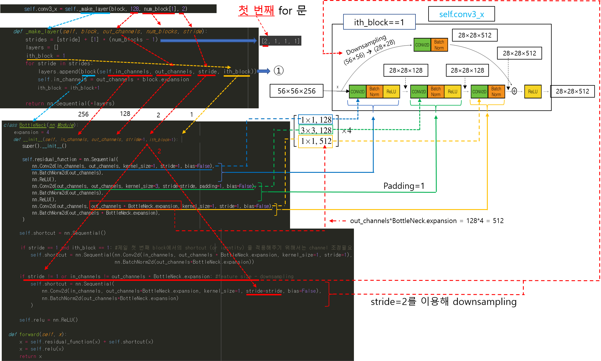
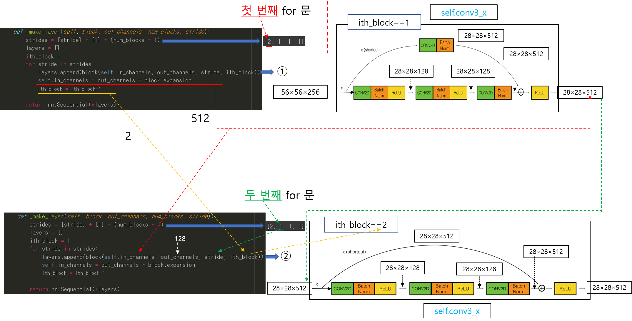
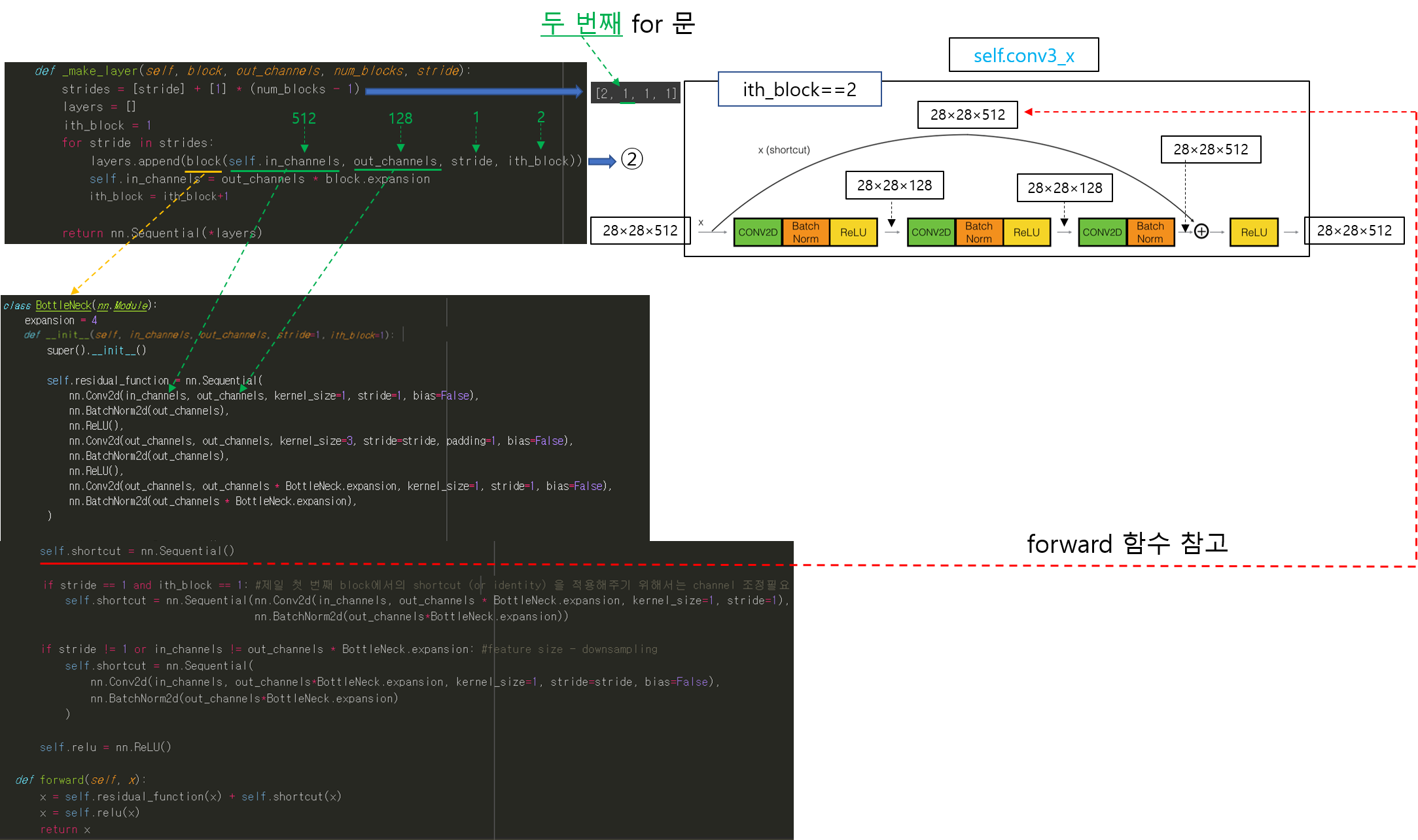
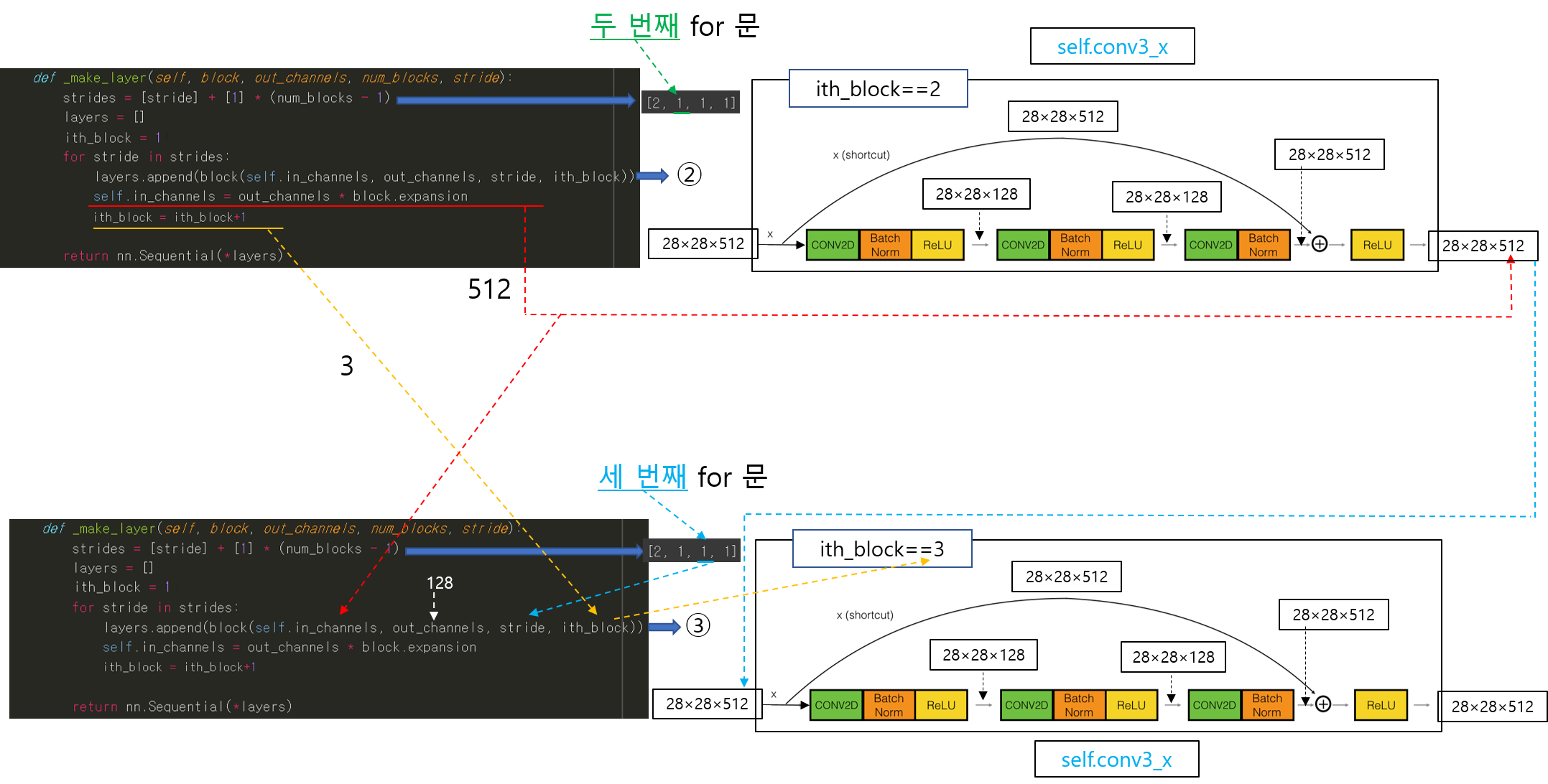
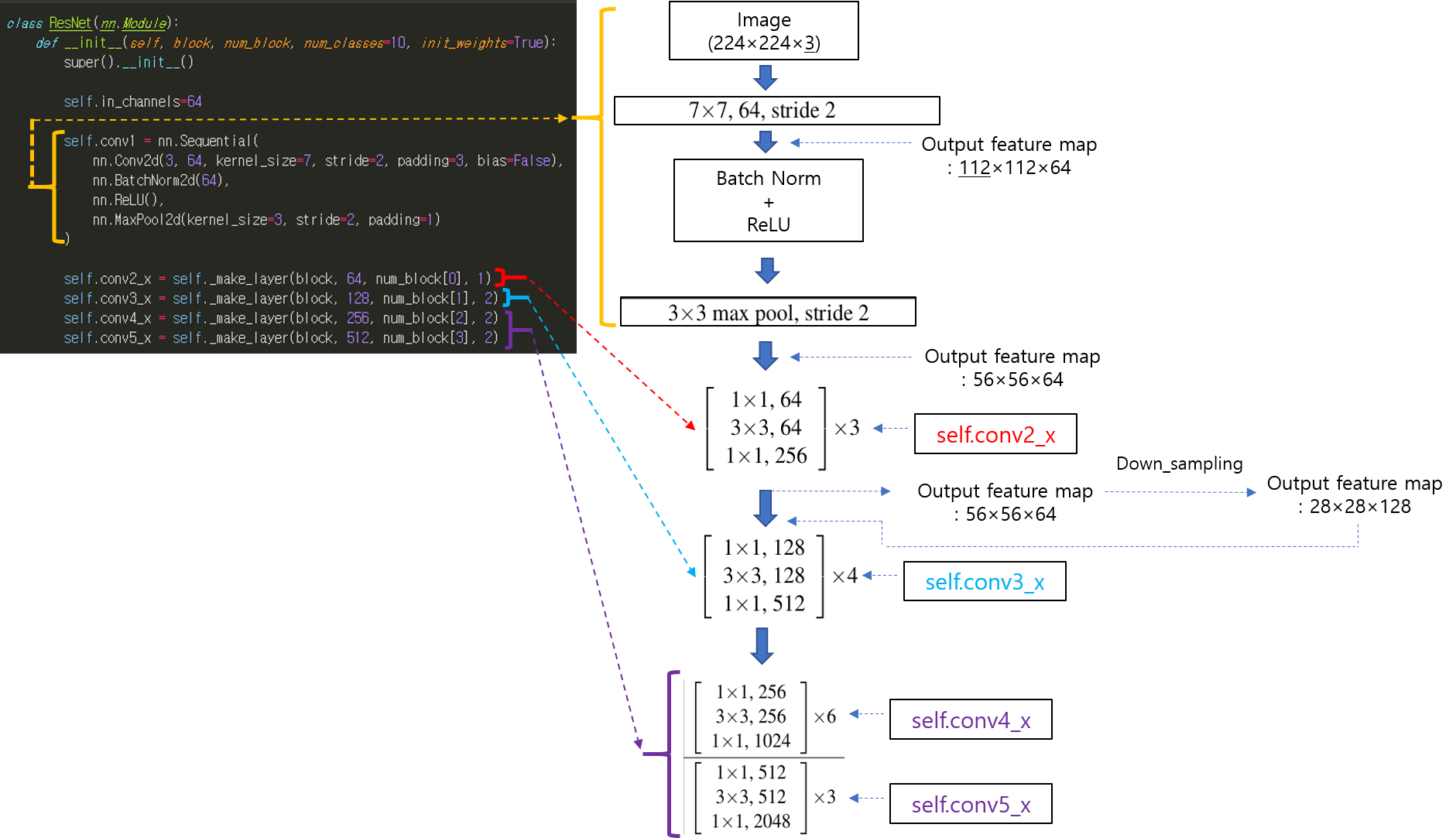
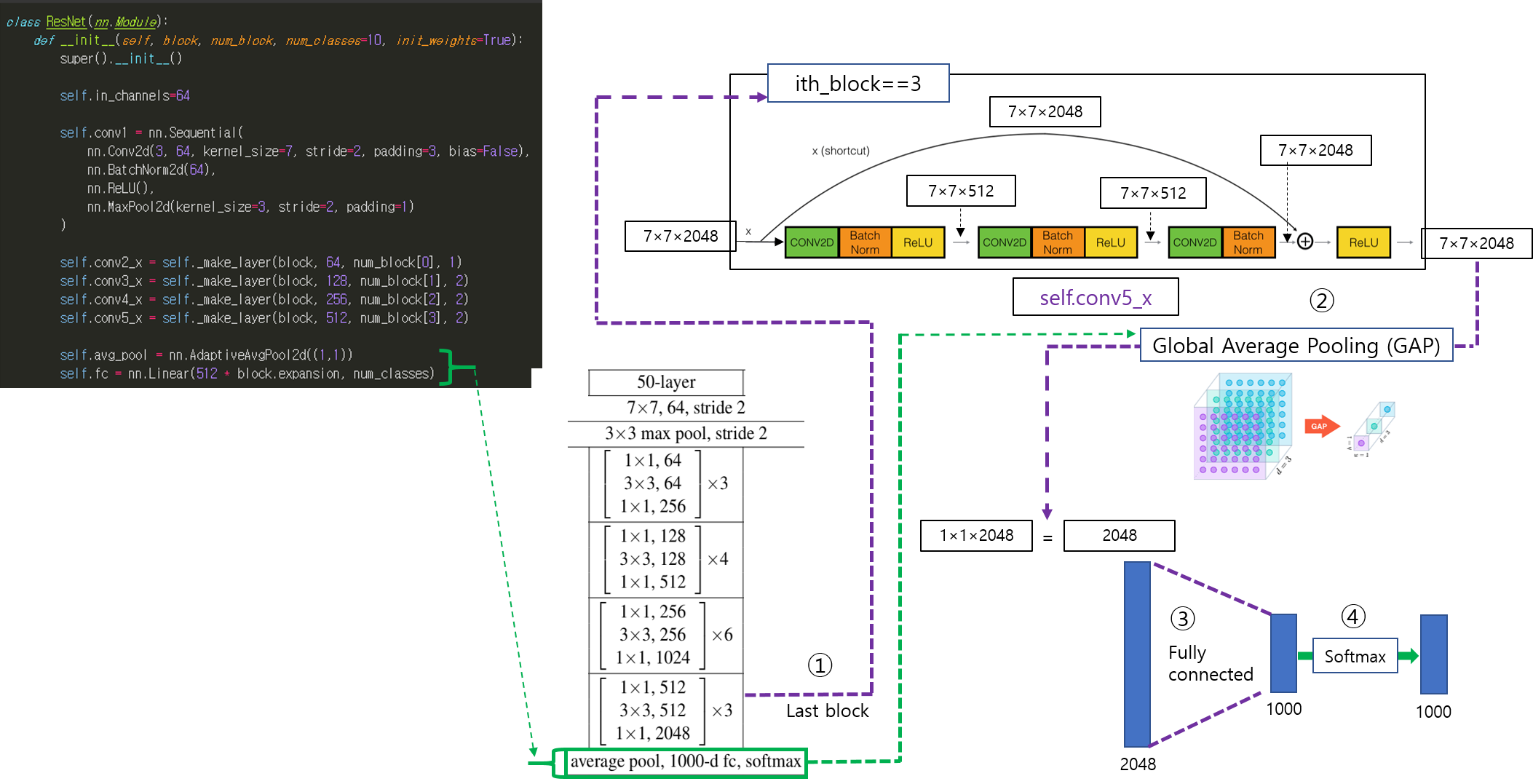
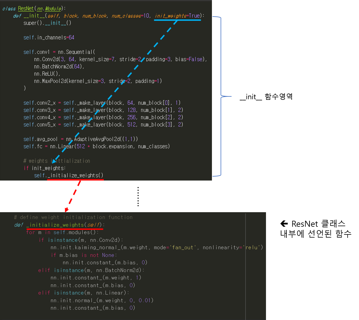
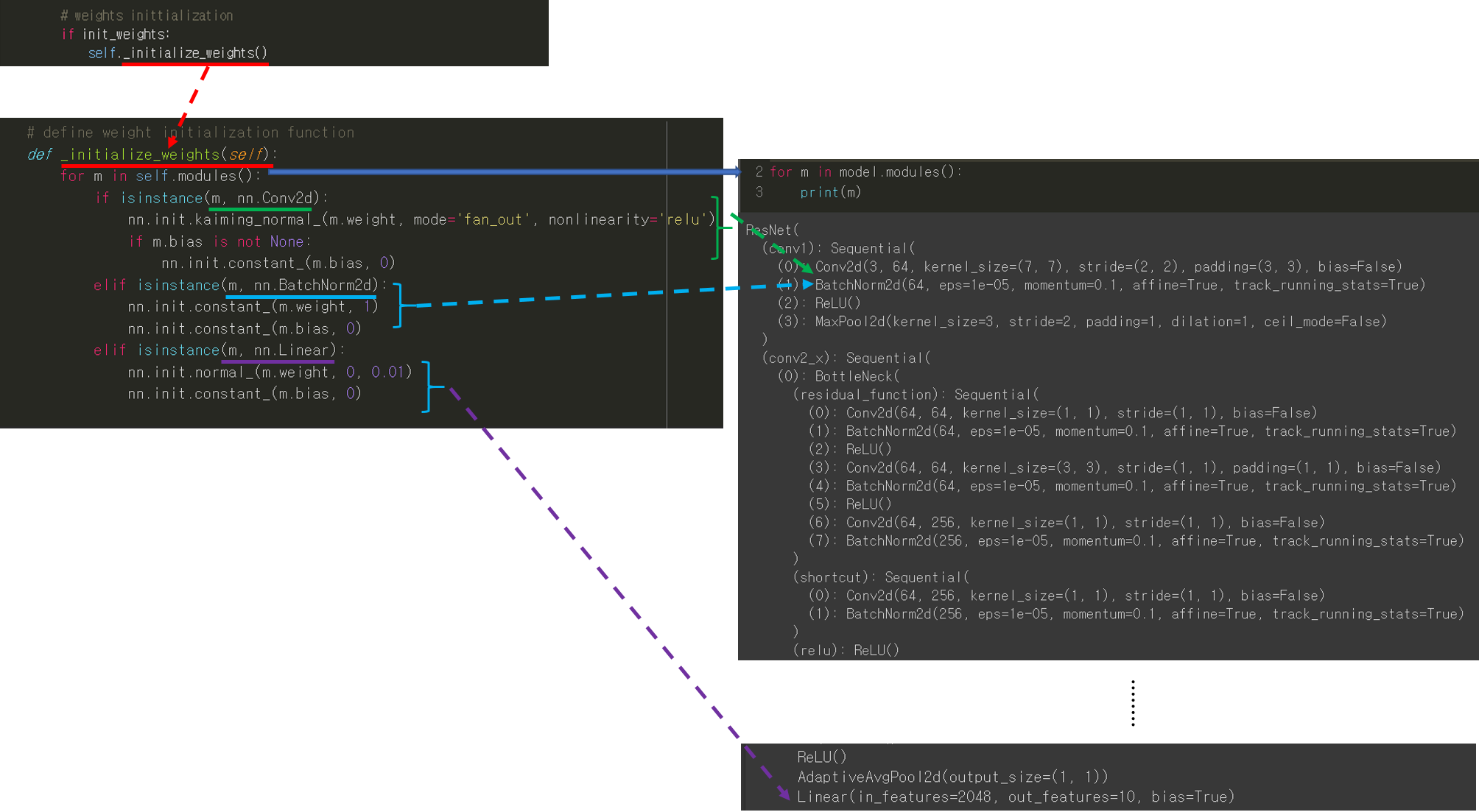
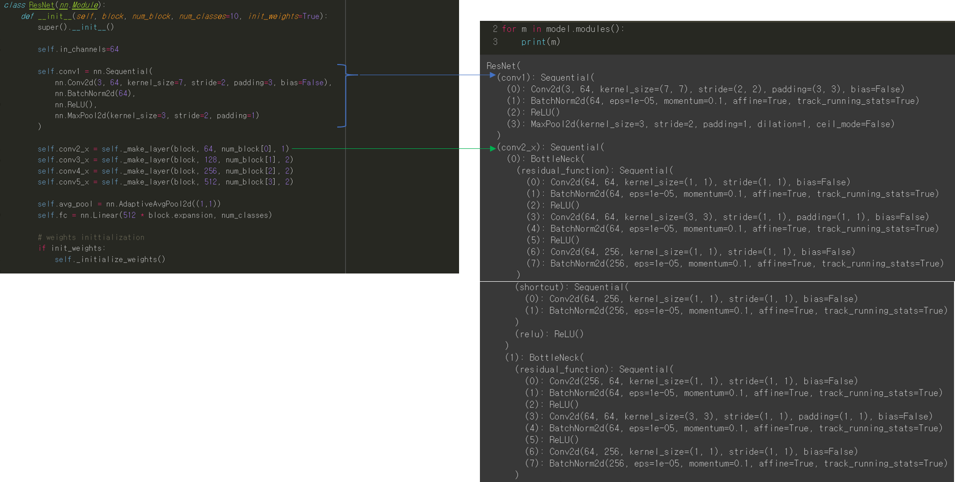
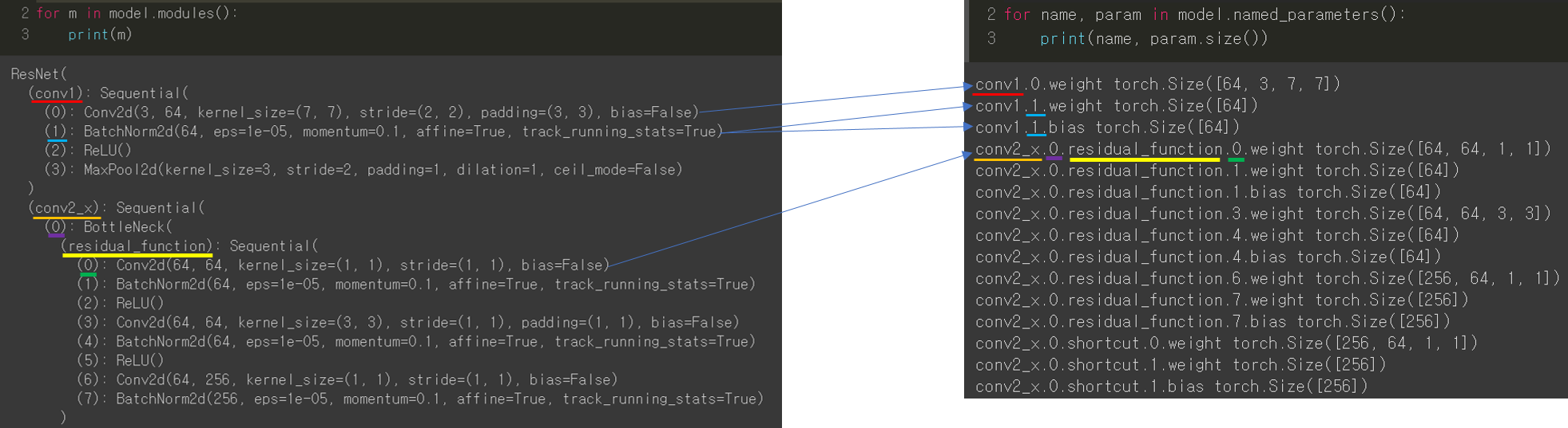
CNN 모델(ResNet)을 처음부터 scratch로 구현해보았습니다.

https://89douner.tistory.com/288?category=994842 

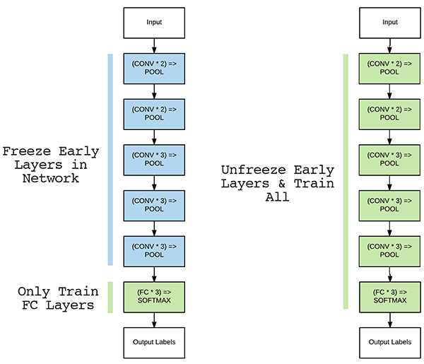
4-4.  Transfer Learning (Feat. Pre-trained model, GPU)

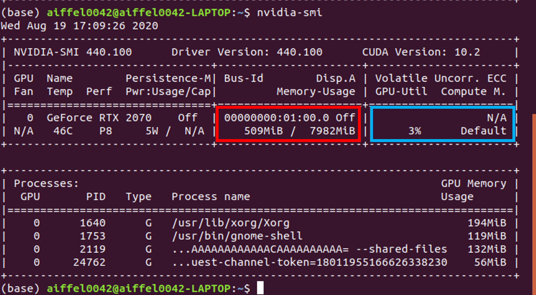
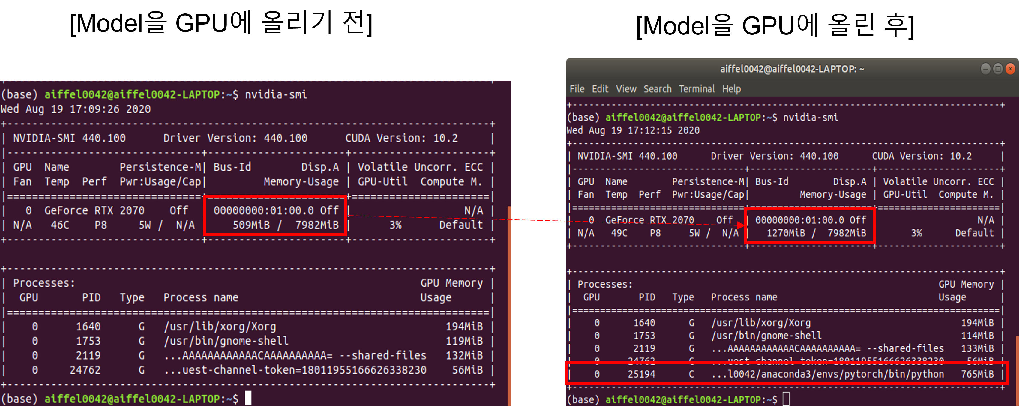
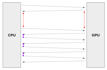
pre-trained model을 다운 받아 transfer learning을 적용하는 코드에 대해서 다루었고, 추가적으로 해당 모델을 GPU에 업로드 하는 것 까지 살펴봤습니다.

https://89douner.tistory.com/289?category=994842 

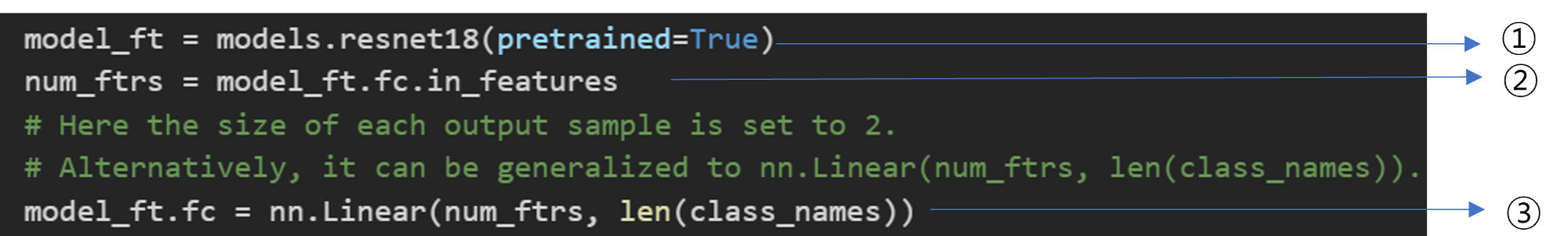
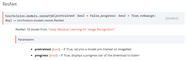
model_ft = models.resnet18(pretrained=True)
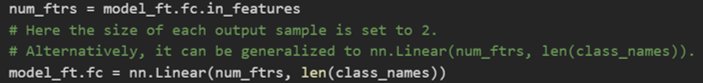
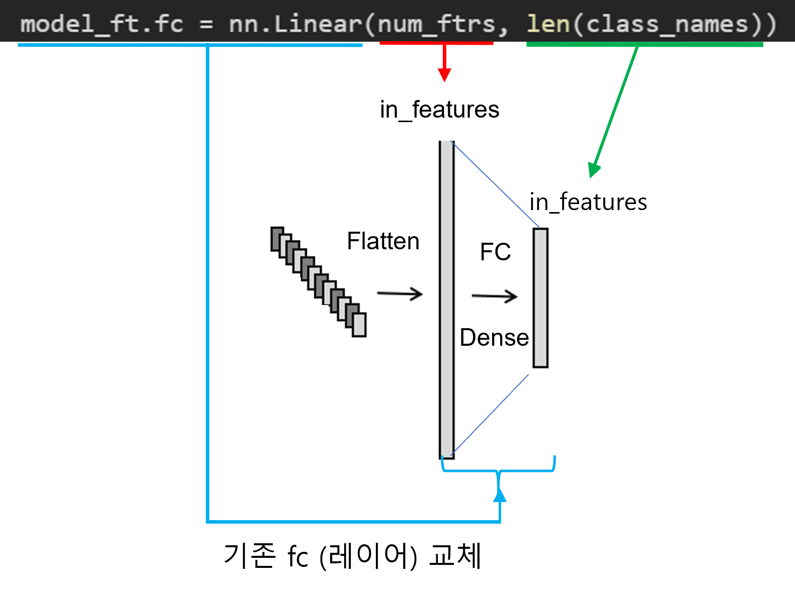
num_ftrs = model_ft.fc.in_features
# Here the size of each output sample is set to 2.
# Alternatively, it can be generalized to nn.Linear(num_ftrs, len(class_names)).
model_ft.fc = nn.Linear(num_ftrs, 2)

model_ft = model_ft.to(device)

4-5.  Loss function, Optimizer, Learning rate policy (← 현재 글)

이번 글에서는 딥러닝 모델이 학습할 방향성에 대해서 정리했고, 관련 코드는 아래와 같습니다.

criterion = nn.CrossEntropyLoss()

# Observe that all parameters are being optimized
optimizer_ft = optim.SGD(model_ft.parameters(), lr=0.001, momentum=0.9)

# Decay LR by a factor of 0.1 every 7 epochs
exp_lr_scheduler = lr_scheduler.StepLR(optimizer_ft, step_size=7, gamma=0.1)

5. 코드 정리

지금까지 배운 내용을 코드로 정리하면 아래와 같습니다.

# License: BSD
# Author: Sasank Chilamkurthy

from __future__ import print_function, division

import torch
import torch.nn as nn
import torch.optim as optim
from torch.optim import lr_scheduler
import numpy as np
import torchvision
from torchvision import datasets, models, transforms
import matplotlib.pyplot as plt
import time
import os
import copy
from warmup_scheduler import GradualWarmupScheduler

plt.ion()   # interactive mode

# Data augmentation and normalization for training
# Just normalization for validation
data_transforms = {
    'train': transforms.Compose([
        transforms.RandomResizedCrop(224),
        transforms.RandomHorizontalFlip(),
        transforms.ToTensor(),
        transforms.Normalize([0.485, 0.456, 0.406], [0.229, 0.224, 0.225])
    ]),
    'val': transforms.Compose([
        transforms.Resize(256),
        transforms.CenterCrop(224),
        transforms.ToTensor(),
        transforms.Normalize([0.485, 0.456, 0.406], [0.229, 0.224, 0.225])
    ]),
}

data_dir = 'data/hymenoptera_data'
image_datasets = {x: datasets.ImageFolder(os.path.join(data_dir, x),
                                          data_transforms[x])
                  for x in ['train', 'val']}
dataloaders = {x: torch.utils.data.DataLoader(image_datasets[x], batch_size=4,
                                             shuffle=True, num_workers=4)
              for x in ['train', 'val']}
dataset_sizes = {x: len(image_datasets[x]) for x in ['train', 'val']}
class_names = image_datasets['train'].classes

device = torch.device("cuda:0" if torch.cuda.is_available() else "cpu")

def imshow(inp, title=None):
    """Imshow for Tensor."""
    inp = inp.numpy().transpose((1, 2, 0))
    mean = np.array([0.485, 0.456, 0.406])
    std = np.array([0.229, 0.224, 0.225])
    inp = std * inp + mean
    inp = np.clip(inp, 0, 1)
    plt.imshow(inp)
    if title is not None:
        plt.title(title)
    plt.pause(0.001)  # pause a bit so that plots are updated


# Get a batch of training data
inputs, classes = next(iter(dataloaders['train']))

# Make a grid from batch
out = torchvision.utils.make_grid(inputs)

imshow(out, title=[class_names[x] for x in classes])

model_ft = models.resnet18(pretrained=True)
num_ftrs = model_ft.fc.in_features
# Here the size of each output sample is set to 2.
# Alternatively, it can be generalized to nn.Linear(num_ftrs, len(class_names)).
model_ft.fc = nn.Linear(num_ftrs, 2)

model_ft = model_ft.to(device)

criterion = nn.CrossEntropyLoss()

# Observe that all parameters are being optimized
optimizer_ft = optim.SGD(model_ft.parameters(), lr=0.001, momentum=0.9) 

# Decay LR by a factor of 0.1 every 3 epochs
exp_lr_scheduler = lr_scheduler.StepLR(optimizer_ft, step_size=3, gamma=0.1)
exp_lr_scheduler = GradualWarmupScheduler(optimizer_ft, multiplier=1, total_epoch=5, after_scheduler=exp_lr_scheduler)

6. 다음 글에서 배울 내용

지금까지 딥러닝 학습을 위한 모든 준비를 끝냈습니다.

그렇다면 딥러닝이 실제로 어떤 단계(code)를 통해 학습하는지 알아봐야겠죠?

이 부분에 대한 내용은 train_model이라는 함수를 통해 실행이 되는데 이 부분은 다음 글에서 살펴보도록 하겠습니다.

(↓↓↓다음 글에서 배울 코드↓↓↓) 

model_ft = train_model(model_ft, criterion, optimizer_ft, exp_lr_scheduler, num_epochs=20)

안녕하세요.

이번 글에서는 transfer learning을 pytorch로 적용하는 방법에 대해서 알아보도록 하겠습니다. 

CNN 모델을 training하는 방식에는 2가지가 있습니다.

1. Scratch training (learning)
   • 자신의 데이터 셋을 기반으로 CNN 모델을 구현하여 학습시키는 방법
   • Scratch training을 하려는 경우에는 지난 글("3.CNN 구현")에서 설명한 방식대로 CNN 모델을 구현하고 자신의 데이터셋을 학습시키면 됩니다. 
2. Transfer learning (← 이번 글에서 설명)
   • ImageNet과 같은 데이터셋으로 학습시킨 CNN 모델을 pre-train 모델이라고 합니다.
   • Transfer learning은 이러한 pre-train 모델을 이용합니다.
   • Pre-trained 모델은 FC layer의 마지막 뉴런 수(=ImageNet 클래스 개수)가 1000 입니다. 그래서, 나의 task가 3개의 class를 분류해야하는 것이라면 FC layer의 마지막 뉴런 수가 3개인 FC layer로 교체해줘야 합니다. (← 자세한 설명은 뒤에서)

그럼 지금부터 transfer learning 적용을 위한 아래 코드들을 하나씩 설명해보도록 하겠습니다.

1. Pre-trained model 다운받기

from torchvision import models

앞선 글("1.Data Load(Feat. CUDA)")에서 torchvision이 크게 3가지 기능을 제공한다고 언급했고, 이 중 2가지인 transforms와 datasets에 대해서 설명드린바 있습니다. 

이번 글에서는 torchvision의 또 다른 기능인 models에 대해 설명드리도록 하겠습니다.

torchvision.models 패키지는 다양한 이미지 task 분야 (ex: classification, dobject detection, segmentation, etc)의 pre-trained 모델을 제공해주고 있습니다.

(↓↓↓classification pre-trained model을 제공해주는 torchvision↓↓↓)

https://pytorch.org/vision/stable/models.html#classification

아래 코드를 입력하면 pre-trained model이 다운받아집니다.

아래 parameters를 보면 알 수 있듯이 pre-trained model은 ImageNet을 기반으로 하고 있는걸 확인할 수 있습니다. 만약 "pretrained=False"로 설정하면 resnet18 모델만 사용할 수 있게 됩니다 (=Conv filter가 학습이 되지 않은 초기화 상태)

2. FC layer 수정해주기

앞서 Pre-trained model을 다운 받았으니 내가 사용할 task에 맞게 FC layer를 변경해주어야 합니다.

import torch.nn as nn

num_ftrs 가 의미하는 바는 아래와 같습니다.

(↓↓↓ResNet 구현된 API↓↓↓)

https://pytorch.org/vision/stable/_modules/torchvision/models/resnet.html#resnet18

"1.Data Load (Feat.CUDA)" 글에서 class_names는 폴더에 있는 클래스 명들을 담고 있다고 했습니다. 만약 분류해야할 클래스가 5개이면 해당 폴더도 5가지로 구성되어 있으니, len(class_name)을 적용하면 5라는 값이 출력 될 것입니다.

3. Fine-tuning 정도 정해주기 (Feat. freezing)

Transfer learning을 적용할 때 상황에 따라 어느 layer까지 학습 가능하게 할지 고려해주어야 합니다.

(↓↓↓Transfer learning을 적용할 때 고려해야할 상황 4가지↓↓↓)

https://89douner.tistory.com/67

Freezing 정도를 pytorch에서는 어떻게 설정해주는지 글로 쓰려고 했는데, 따로 정리한 PPT에 설명이 잘되어 있어서 아래 PPT 자료로 설명을 대체하겠습니다. (파일 용량이 10MB 이상 업로드가 안돼서 디자인도 바꾸고 중간중간 슬라이드 부분도 제거해버렸네요 ㅜㅜ)

또한 특정 layer의 conv filter 또는 batch normalization의 beta, gamma 값을 초기화(initialization) 해주어야 할 때도 있습니다. 이러한 경우 어떻게 초기화 시키면 되는지 또한 PPT 자료로 정리해놨으니 참고해주시면 감사하겠습니다 (파일 용량이 10MB 이상 업로드가 안돼서 디자인도 바꾸고 중간중간 슬라이드 부분도 제거해버렸네요 ㅜㅜ)

(↓↓↓batch norm gamma, beta 초기화 필요성을 언급한 논문↓↓↓)

https://89douner.tistory.com/248?category=908624 

3. Model을 GPU에 업로드 하기

학습하기 위해 모델 구축을 마무리 했습니다. 그럼 실제 학습을 위해 이제부터 딥러닝 model을 GPU에 올려놓도록 하겠습니다.

아직 model을  GPU에 올리기 전 상태이기 때문에, nvidia-smi를 통해 GPU 메모리를 확인하면 대략 500MiB의 메모리가 다른 OS 관련 process를 잡고 있는걸 볼 수 있습니다. (GPU-Util (=GPU 이용율) 부분도 3%이므로 GPU가 거의 쉬고 있다고 보시면 됩니다)

아래와 같이 코드를 수행해도 GPU 상의 메모리를 확인할 수 있는데, 아래 코드를 이용하면 아무런 메모리도 올라가 있지 않다는걸 확인할 수 있습니다. torch 관련한 코드로 GPU 메모리를 확인하면 torch 코드로 GPU 상에 데이터를 업로드 하지 않은 이상 GPU 메모리 용량이 0으로 표현되는듯 합니다.

이번엔 아래 코드를 수행하여 딥러닝 모델을 GPU에 업로드 하고, GPU 메모리를 확인해 보도록 하겠습니다.

• model.to(device): When loading a model on a GPU that was trained and saved on GPU, simply convert the initialized model to a CUDA optimized model using model.to(torch.device('cuda')).

• torch.cuda.memory_allocated 설명
  • You can use memory_allocated() and max_memory_allocated() to monitor memory occupied by tensors, and use memory_reserved() and max_memory_reserved() to monitor the total amount of memory managed by the caching allocator.
• torch.cuda.memory_cached 설명
  • PyTorch uses a caching memory allocator to speed up memory allocations.
  • This allows fast memory deallocation without device synchronizations.

• However, the unused memory managed by the allocator will still show as if used in nvidia-smi.
  
  • The nvidia-smi number includes space the allocated by the CUDA driver when it loads PyTorch.
  • This can be quite large because PyTorch includes many CUDA kernels. On a P100, I’ve seen an overhead of ~487 MB.
  • This memory isn’t reported by the torch.cuda.xxx_memory functions because it’s not allocated by the program and there isn’t a good way to measure it outside of looking at nvidia-smi.
  • Our tensor is too small. The caching allocator allocates memory with a minimum size and a block size so it may allocate a bit more memory than the number of elements in your tensors.
  • Things like cuda ctx, cuda rng state, cudnn ctx, cufft plans, and other gpu memory your other libraries may use are not counted in the torch.cuda.* stats.

지금까지 배운 내용(1.Data load(Feat. CUDA), 2.Data Preprocessing(Feat. Augmentation))을 코드로 요약 하면 아래와 같습니다.

# License: BSD
# Author: Sasank Chilamkurthy

from __future__ import print_function, division

import torch
import torch.nn as nn
import torch.optim as optim
from torch.optim import lr_scheduler
import numpy as np
import torchvision
from torchvision import datasets, models, transforms
import matplotlib.pyplot as plt
import time
import os
import copy

plt.ion()   # interactive mode

# Data augmentation and normalization for training
# Just normalization for validation
data_transforms = {
    'train': transforms.Compose([
        transforms.RandomResizedCrop(224),
        transforms.RandomHorizontalFlip(),
        transforms.ToTensor(),
        transforms.Normalize([0.485, 0.456, 0.406], [0.229, 0.224, 0.225])
    ]),
    'val': transforms.Compose([
        transforms.Resize(256),
        transforms.CenterCrop(224),
        transforms.ToTensor(),
        transforms.Normalize([0.485, 0.456, 0.406], [0.229, 0.224, 0.225])
    ]),
}

data_dir = 'data/hymenoptera_data'
image_datasets = {x: datasets.ImageFolder(os.path.join(data_dir, x),
                                          data_transforms[x])
                  for x in ['train', 'val']}
dataloaders = {x: torch.utils.data.DataLoader(image_datasets[x], batch_size=4,
                                             shuffle=True, num_workers=4)
              for x in ['train', 'val']}
dataset_sizes = {x: len(image_datasets[x]) for x in ['train', 'val']}
class_names = image_datasets['train'].classes

device = torch.device("cuda:0" if torch.cuda.is_available() else "cpu")

def imshow(inp, title=None):
    """Imshow for Tensor."""
    inp = inp.numpy().transpose((1, 2, 0))
    mean = np.array([0.485, 0.456, 0.406])
    std = np.array([0.229, 0.224, 0.225])
    inp = std * inp + mean
    inp = np.clip(inp, 0, 1)
    plt.imshow(inp)
    if title is not None:
        plt.title(title)
    plt.pause(0.001)  # pause a bit so that plots are updated


# Get a batch of training data
inputs, classes = next(iter(dataloaders['train']))

# Make a grid from batch
out = torchvision.utils.make_grid(inputs)

imshow(out, title=[class_names[x] for x in classes])

model_ft = models.resnet18(pretrained=True)
num_ftrs = model_ft.fc.in_features
# Here the size of each output sample is set to 2.
# Alternatively, it can be generalized to nn.Linear(num_ftrs, len(class_names)).
model_ft.fc = nn.Linear(num_ftrs, 2)

model_ft = model_ft.to(device)

다음 글에서는 딥러닝 모델이 학습할 방향성을 결정해주는 loss function, optimizer, learning rate schedule 에 대해서 알아보도록 하겠습니다.

(↓↓↓ 다음 글에서 배울 코드내용↓↓↓)

criterion = nn.CrossEntropyLoss()

# Observe that all parameters are being optimized
optimizer_ft = optim.SGD(model_ft.parameters(), lr=0.001, momentum=0.9)

# Decay LR by a factor of 0.1 every 7 epochs
exp_lr_scheduler = lr_scheduler.StepLR(optimizer_ft, step_size=7, gamma=0.1)

안녕하세요.

이번 글에서는 pytorch를 이용해서 대표적인 CNN 모델인 ResNet을 implementation 하는데 필요한 코드를 line by line으로 설명해보려고 합니다.

ResNet을 구현할 줄 아시면 전통적인 CNN 모델들은 자유롭게 구현하는데 어려움이 없을거라 생각됩니다. 

우선 pytorch에서 resnet 모델을 불러오는 코드는 아래 한 줄로 가능합니다.

model = resnet50().to(device)

그렇다면 resnet50() 이라는 함수가 어떤 과정을 통해 실행되는지 살펴봐야겠죠?

지금부터 이 과정을 순차대로 살펴보도록 하겠습니다.

※ 최종코드는 제일 아래에 있으니 참고해주세요!

※ 대부분 PPT 슬라이드에 설명한 내용을 이미지로 만들어 업로드했기 때문에 글씨가 잘 안보일 수도 있습니다. 그래서 PPT파일을 따로 첨부 하도록 하겠습니다.

0. ResNet() 함수 호출

• 먼저 resnet50()을 호출하면 ResNet(BottleNeck, [3,4,6,3]) 함수를 호출하게됩니다.
• ResNet 함수 내부를 대략적으로 살펴보면 ResNet50 구조를 파악할 수 있습니다.

1. (BottleNeck 적용 전) 첫 번째 conv layer

• ResNet 함수에서 첫 번째 conv layer 부터 살펴보도록 하겠습니다.

2. 두 번째 Conv layer

• 두 번째 Conv layer 부터 bottleneck이 적용됩니다. 앞서 노란색 영역인 첫 번째 conv layer를 지나면, 아래 빨간색 영역의 첫 번째 bottleneck 연산이 진행됩니다.
• 우선 첫 번째 bottleneck을 간단히 도식화하면 아래와 같이 나타낼 수 있습니다.

• Bottleneck이 포함된 conv layer를 생성하기 위해 make_layer 함수가 실행되야 하는데, make_layer 함수에 작성된 python 기본 문법들을 먼저 설명하겠습니다. 
  • 연산자를 이용한 리스트 생성
  • for in 반복문 (with 리스트)
  • 리스트 인자 함수
  • Sequential 함수

• sequential 함수 설명

2-1. 두 번째 Conv layer에서 첫 번째 BottleNeck 적용 (make_layer(), BottleNeck()=block() 함수 호출)

2-2. 두 번째 Conv layer에서 두 번째 BottleNeck 적용 (make_layer(), BottleNeck()=block() 함수 호출)

2-3. 두 번째 Conv layer에서 세 번째 BottleNeck 적용 (make_layer(), BottleNeck()=block() 함수 호출)

3. 세 번째 Conv layer

3-1. 세 번째 Conv layer에서 첫 번째 BottleNeck 적용 (make_layer(), BottleNeck()=block() 함수 호출 + Down_sampling)

• 여기서 부터는 첫 번째 bottleNeck에 shortcut (for skip connection) 적용을 위해 down_sampling이 된다는 점을 알아두시면 좋을 것 같습니다.
• Down_sampling은 conv filter의 stride를 2로 설정함으로써 진행이 됩니다.

3-2. 세 번째 Conv layer에서 두 번째 BottleNeck 적용 (make_layer(), BottleNeck()=block() 함수 호출)

3-3. 세 번째 Conv layer에서 세 번째 BottleNeck 적용 (make_layer(), BottleNeck()=block() 함수 호출)

• block 함수 부분은 이전과 설명이 동일 하므로 이제부터는 생략하겠습니다.

3-4. 세 번째 Conv layer에서 세 번째 BottleNeck 적용 (make_layer(), BottleNeck()=block() 함수 호출)

4, 5. 네 번째 Conv layer, 다섯 번째 Conv layer

• 여기서부터는 위에서 설명한 내용의 반복이라 make_layer, block 함수 실행과정은 생략하도록 하겠습니다.

6. Average pooling, FC layer, Softmax

7. Weight initialization

(↓↓↓ 가중치 초기화 관련 API ↓↓↓)

https://pytorch.org/docs/stable/nn.init.html

8. Model Show

• 앞서 작성한 코드가 올바로 작성됐는지 해당 모델 구조를 들여다보는 세 가지 방법에 대해서 알아보겠습니다.

8-1. model.modules()

8-2. model.named_parameters()

8-3. summary()

9. 최종 코드

# model
import torch
import torch.nn as nn
import torch.nn.functional as F
from torchsummary import summary

class ResNet(nn.Module):
    def __init__(self, block, num_block, num_classes=10, init_weights=True):
        super().__init__()

        self.in_channels=64

        self.conv1 = nn.Sequential(
            nn.Conv2d(3, 64, kernel_size=7, stride=2, padding=3, bias=False),
            nn.BatchNorm2d(64),
            nn.ReLU(),
            nn.MaxPool2d(kernel_size=3, stride=2, padding=1)
        )

        self.conv2_x = self._make_layer(block, 64, num_block[0], 1)
        self.conv3_x = self._make_layer(block, 128, num_block[1], 2)
        self.conv4_x = self._make_layer(block, 256, num_block[2], 2)
        self.conv5_x = self._make_layer(block, 512, num_block[3], 2)

        self.avg_pool = nn.AdaptiveAvgPool2d((1,1))
        self.fc = nn.Linear(512 * block.expansion, num_classes)

        # weights inittialization
        if init_weights:
            self._initialize_weights()

    def _make_layer(self, block, out_channels, num_blocks, stride):
        strides = [stride] + [1] * (num_blocks - 1)
        layers = []
        ith_block = 1
        for stride in strides:
            layers.append(block(self.in_channels, out_channels, stride, ith_block))
            self.in_channels = out_channels * block.expansion
            ith_block = ith_block+1

        return nn.Sequential(*layers)

    def forward(self,x):
        output = self.conv1(x)
        output = self.conv2_x(output)
        x = self.conv3_x(output)
        x = self.conv4_x(x)
        x = self.conv5_x(x)
        x = self.avg_pool(x)
        x = x.view(x.size(0), -1)
        x = self.fc(x)
        return x

    # define weight initialization function
    def _initialize_weights(self):
        for m in self.modules():
            if isinstance(m, nn.Conv2d):
                nn.init.kaiming_normal_(m.weight, mode='fan_out', nonlinearity='relu')
                if m.bias is not None:
                    nn.init.constant_(m.bias, 0)
            elif isinstance(m, nn.BatchNorm2d):
                nn.init.constant_(m.weight, 1)
                nn.init.constant_(m.bias, 0)
            elif isinstance(m, nn.Linear):
                nn.init.normal_(m.weight, 0, 0.01)
                nn.init.constant_(m.bias, 0)


def resnet50():
    return ResNet(BottleNeck, [3,4,6,3])

class BottleNeck(nn.Module):
    expansion = 4
    def __init__(self, in_channels, out_channels, stride=1, ith_block=1):
        super().__init__()

        self.residual_function = nn.Sequential(
            nn.Conv2d(in_channels, out_channels, kernel_size=1, stride=1, bias=False),
            nn.BatchNorm2d(out_channels),
            nn.ReLU(),
            nn.Conv2d(out_channels, out_channels, kernel_size=3, stride=stride, padding=1, bias=False),
            nn.BatchNorm2d(out_channels),
            nn.ReLU(),
            nn.Conv2d(out_channels, out_channels * BottleNeck.expansion, kernel_size=1, stride=1, bias=False),
            nn.BatchNorm2d(out_channels * BottleNeck.expansion),
        )

        self.shortcut = nn.Sequential()

        if stride == 1 and ith_block == 1: #첫 번째 block에서의 shortcut (or identity) 을 적용해주기 위해서는 channel 조정필요
            self.shortcut = nn.Sequential(nn.Conv2d(in_channels, out_channels * BottleNeck.expansion, kernel_size=1, stride=1), 
                                          nn.BatchNorm2d(out_channels*BottleNeck.expansion))

        if stride != 1 or in_channels != out_channels * BottleNeck.expansion: #feature size_downsampling
            self.shortcut = nn.Sequential(
                nn.Conv2d(in_channels, out_channels*BottleNeck.expansion, kernel_size=1, stride=stride, bias=False),
                nn.BatchNorm2d(out_channels*BottleNeck.expansion)
            )
            

        self.relu = nn.ReLU() 

    def forward(self, x):
        x = self.residual_function(x) + self.shortcut(x)
        x = self.relu(x)
        return x

device = torch.device('cuda' if torch.cuda.is_available() else 'cpu')
model = resnet50().to(device)
x = torch.randn(3, 3, 224, 224).to(device)
output = model(x)
print(output.size())

for name, param in model.named_parameters():
    print(name, param.size())

for m in model.modules():
    print(m)

#ResNet50 모델 summary 
summary(model, (3, 224, 224), device=device.type)

지금까지 ResNet50을 pytorch로 구현한 code에 대해서 설명해봤습니다.

다음 글에서는 Pretrained model를 불러드려와 transfer learning을 적용시키는 코드에 대해 설명하도록 하겠습니다.

안녕하세요.

지난 글에서 torchvision.transforms를 설명하면서 pytorch가 기본적인 augmentation 기법을 제공해준다고 언급한바 있습니다.

하지만, 기본적인 augmentation 외에도 다양한 영역에서 특수하게 사용하는 독특한 augmentation 기법들이 존재합니다. 예를 들어, Chest X-ray 데이터에는 N-CLAHE라는 독특한 전처리 기법이 있는데, 이러한 전처리 기법은 pytorch에서 기본으로 제공되고 있지 않습니다.

그러므로 별도의 augmentation 패키지를 이용하여 pytorch에 적용해야 합니다. (← transforms.Compose에 연동)

이번 글에서는 두 가지 augmentation 패키지에 대해서 소개하려고 합니다.

1. imgaug 패키지

https://github.com/aleju/imgaug

https://uos-deep-learning.tistory.com/17

2. albumentations 패키지

https://hoya012.github.io/blog/albumentation_tutorial/

https://deep-learning-study.tistory.com/673

albumentations 패키지 관련해서는 segmentation 카테고리에 설명해놨으니 위에 있는 사이트와 더불어 같이 보시면 구현하시기 편하실 거에요!

https://89douner.tistory.com/312

안녕하세요.

이번 글에서는 CNN 모델 학습을 위해 학습 데이터들을 로드하는 코드에 대해 설명드리려고 합니다.

아래 사이트의 코드를 기반으로 설명드리도록 하겠습니다.

https://pytorch.org/tutorials/beginner/transfer_learning_tutorial.html

우선 데이터를 로드하는 과정을 총 6단계로 나누어 설명하도록 하겠습니다.

from torchvision import datasets, models, transforms

위의 코드를 보면 torchvision에서 transforms, datasets 이라는 패키지가 사용되었다는걸 확인할 수 있습니다. Pytorch에는 torchvision이라는 패키지를 이용해 다양한 computer vision 관련 task를 수행할 수 있습니다. 각각의 패키지들 (datasets, transforms, models) 에 대해서는 위의 코드를 분석하면서 같이 설명하도록 하겠습니다.

https://pytorch.org/vision/stable/index.html

1. transforms (Feat. Data Augmentation)

•  transforms라는 패키지는 말 그대로 이미지를 transformation (=augmentation) 해주는 기능들을 제공해주고 있습니다.
• 우리가 augmentation을 하기 위한 crop, resize, flip 등은 모두 이미지에 transformation이 적용된 상태입니다.

https://pytorch.org/vision/stable/transforms.html

from torchvision import transforms

• 위의 코드를 살펴보면 compose 함수인자에 transforms 객체들의 list를 입력 받습니다.
• 이것이 의미하는 바가 무엇일까요? 계속해서 알아보도록 하겠습니다. 

• data_transforms 자체는 dictionary로 정의되었습니다.
• 그리고 각 key에 해당 하는 value 값은 클래스 객체 Compose인 것을 알 수 있습니다.
• Compose 객체에 다양한 인자 값들이 포함되어 있는데, 이 인자 값들이 augmentation이 적용되는 순서라고 보시면 됩니다.
• EX) data_tranforms['train']의 경우
  1. RandomResizedCrop 수행
     • scale → Specifies the lower and upper bounds for the random area of the crop, before resizing. The scale is defined with respect to the area of the original image.
     • ratio → lower and upper bounds for the random aspect ratio of the crop, before resizing.
  2. RandomHorizontalFlip 수행
     • p=0.5 → 50%의 확률로 RandomHorizontalFlip 실행
  3. ToTensor 수행
     • 처음 로드되는 이미지 형태를 딥러닝 학습 format에 맞는 tensor 형태로 변경
     • Converts a PIL Image or numpy.ndarray (H x W x C) in the range [0, 255] to a torch.FloatTensor of shape (C x H x W) in the range [0.0, 1.0]
  4. Normalize 수행
     • 이미지 전처리 (Preprocessing)
     • Normalization에 들어가는 값들이 어떻게 계산되는지는 아래 PPT를 참고해주세요.

2. datasets(Feat. Data Augmentation)

• datasets.ImageFolder를 이용하면 이미지 디렉터리에 존재하는 이미지 메타정보 (ex: 이미지 개수, augmentation 기법들, etc..) 등을 하나의 tuple 형태로 저장할 수 있습니다 ← ImageFolder의 return 형태는 tuple
• 나중에 DataLoader를 이용해 실제 이미지를 load 할 때, 이미지 메타정보(=tuple 형태)들을 이용해 쉽게 load할 수 있습니다 ← 뒤에서 설명    
  • root: Root directory of dataset 
  • transforms:  A function/transform that takes in an PIL image and returns a transformed version (ex: transforms.RandomCrop)

from torchvision import datasets
import os

※os.path.join 함수 예시 ↓↓↓

• 아래 결과를 보면 이미지 폴더의 메타정보들을 확인할 수 있습니다.
  • 'train': Dataset Image Folder
  • Number of datapoints: train 폴더에 들어있는 총 이미지 개수
  • Transform: 적용될 augmentation 순서 

https://pytorch.org/vision/stable/datasets.html

• 아래 코드는 dictionary 자료형을 for 문으로 만드는 문법입니다.

• dataset_size 변수는 딥러닝 모델(CNN)을 학습 시킬 때 epoch 단위의 loss or accuracy 산출을 위해 이용됩니다. (자세한 설명은 train을 구현하는 함수에서 설명하도록 하겠습니다)

• train 폴더를 보면 총 5개의 class가 있다는걸 확인 할 수 있습니다.
• image_datasets['train'].classes을 이용하면 아래 폴더를 기준으로 class 명들을 string 형태로 사용할 수 있게 됩니다.

※이번 코드에서는 포함되어 있진 않지만, datasets 패키지의 첫 번째 활용도는 cifar10, caltech101, imagenet 과 같이 범용적으로 쓰이는 데이터를 쉽게 다운로드 받아 이용할 수 있게 해준다는 점입니다. 상식으로 알아두시면 좋습니다!

3. DataLoader

• At the heart of PyTorch data loading utility is the torch.utils.data.DataLoader class.
• 딥러닝에서 이미지를 load 하기 위해서는 batchsize, num_workers 등의 사전 정보들을 정의해야합니다. (※torch.utils.data.DataLoader가 이미지를 GPU에 업로드 시켜주는 코드가 아니라, 사전 정보들을 정의하는 역할만 한다는 것을 알아두세요!) 
  • image_datasets[x]: 예를 들어, image_datasets['train']인 경우 train 폴더에 해당하는 클래스들의 이미지 경로를 설정해줍니다.
  • batch_size: 학습을 위한 batch size 크기를 설정해줍니다.
  • shuffle: 이미지 데이터를 불러들일 때, shuffle을 적용 여부를 설정해줍니다.
  • num_workers: 바로 아래에서 따로 설명
• 아래 코드 역시 dataloaders라는 dictionary 형태의 변수를 for 문으로 생성하는 코드 입니다. 

[num_workers]

• 학습 이미지를 GPU에 할당시켜 주기 위해서는 CPU의 조력이 필요합니다. 즉, CPU가 학습 이미지를 GPU에 올려주는 역할을 하는 것이죠.
• 좀 더 구체적으로 말하자면, CPU에서 process 생성해 학습 이미지를 GPU에 업로드 시켜주는 방식입니다.
• num_workers는 CPU가 GPU에 이미지를 업로드 할 때, 얼마나 많은 subprocess를 이용할지를 결정하는 인자(argument)라고 생각하시면 됩니다. 
  • how many subprocesses to use for data loading. 0 means that the data will be loaded in the main process. (default: 0)

(↓↓↓process 관련해서 정리해 놓은 글↓↓↓)

https://89douner.tistory.com/150

• 만약 num_workers를 적게 설정하면 어떻게 될까요?
  • num_workers를 0으로 설정했을 때 (=a main process), CPU가 하나의 이미지를 GPU에  업로드 하는 시간을 1초라고 가정해보겠습니다.
  • 이 때, 업로드된 이미지를 GPU에서 처리 (for CNN training) 를 하는 것이 0.1초라고 가정한다면, 다음 이미지를 업로드 할 때 까지 0.9초 동안 GPU는 놀게(idle)됩니다. (아래 "그림14"에서 빨간색 간격 → CPU에서 GPU로 이미지 데이터를 넘기기 위해 수행되는 전처리 과정)
• 결국 CPU에서 GPU로 이미지를 넘겨주는 작업을 빠르게 증가시키기 위해서는 여러 subprocess를 이용해 이미지들을 GPU에 업로드 시켜주어야 합니다. 다시 말해, 다수의 process를 이용해서 CPU에서 GPU로 이미지 데이터를 넘기기 위한 전처리 시간을 축소시켜주는 것이죠.
• 이렇게 num_workers를 증가하여 GPU에 이미지를 업로드 시키는 속도가 빨라지면, GPU가 놀지 않고 열심히 일하게 될 것입니다. → GPU 사용량(이용률)이 증가하게 된다고도 할 수 있습니다. 
  • More num_workers would consume more memory usage but is helpful to speed up the I/O process.

• 하지만, CPU가 GPU에 이미지를 업로드 시켜주는 역할은 수 많은 CPU의 역할 중 하나입니다.
• 즉, num_workers를 너무 많이 설정해주어 CPU코어들을 모두 dataload에 사용하게 되면, CPU가 다른 중요한 일들을 못하게 되는 상황이 발생되는 것이죠.
  • CPU의 코어 개수는 물리적으로 한정되어 있습니다.

(↓↓↓Core(코어)에 대한 개념을 정리한 글↓↓↓)

https://89douner.tistory.com/151

• num_workers를 어떻게 설정하면 좋은지에 대해서는 pytorch forum에서도 다양한 의견들이 나오고 있습니다.

https://discuss.pytorch.org/t/guidelines-for-assigning-num-workers-to-dataloader/813

• 보통 코어 개수의 절반 정도로 num_workers를 설정하는 경우도 있지만, 보통 batch size를 어떻게 설정해주냐에 따라서 num_workers를 결정해주는 경우가 많습니다. 
• 경험적으로 batch_size가 클 때, num_workers 부분도 크게 잡아주면 out of memory 에러가 종종 발생해서, num_workers 부분을 줄이거나, batch_size 부분을 줄였던 것 같습니다. (이 부분은 차후에 다시 정리해보도록 하겠습니다.)

※num_workers에 대한 설명은 아래 reference를 참고했습니다.

https://jybaek.tistory.com/799

• torch.utils.data.Dataloader를 통해 생성한 dataloaders 정보들을 출력하면 아래와 같습니다.

4. GPU에 업로드 될 이미지 확인하기

앞서 "torch.utils.data.DataLoader"를 통해 이미지를 GPU에 올릴 준비를 끝냈으니, 어떤 이미지들의 GPU에 올라갈 지 확인해보겠습니다.

inputs에 어떤 정보들이 저장되어 있는지 알아보도록 하겠습니다.

• inputs 데이터에는 batch 단위로 이미지들이 저장되어 있는 것을 확인할 수 있습니다.

• 앞서 dataset_sizes['train'] 에서 확인 했듯이, train 원본 이미지 개수는 ‘2683’개 입니다.
• transformer.compose()를 통해 생성된 train 이미지 개수도 ‘2683’개 이다.
• imshow를 통해 생성된 이미지를 봤을 때, data augmentation에 의해 데이터 수가 늘어난게 아니라, 본래 2683개의 데이터 자체내에서 augmentation이 적용된 것 같습니다. 다시 말해, training dataset의 (절대)개수는 data augmentation을 적용했다고 해서 늘어나는 것이 아닙니다. (imshow 함수는 이 글 제일 아래 있습니다)
• 결국, (inputs, classes) 가 CNN 입장에서 (학습 이미지 데이터, 라벨) 정보를 담고 있다고 볼 수 있겠네요.

• 하지만, 딥러닝 입장에서 중복된 데이터는 학습을 위해 큰 의미가 없을 가능성이 높습니다. 그래서 이미지A 5장이 있는것과, 이미지 A에 5가지 augmentation 적용된 것을 학습한다고 했을 때, 딥러닝 입장에서는 후자의 경우 더 많은 데이터가 있다고 볼 수 있습니다.
• 그래서 위와 같이 첫 번째 epoch의 첫 번째 iteration에서 잡힌 4개(batch) 이미지에 적용된 augmentation과, 두 번째 iteration에서 잡힌 4개(batch) 이미지에 적용된 augmentation과 다르기 때문에 결국 epoch을 여러 번 진행해주게되면, 다양한 조합으로 data augmentation이 적용되기 때문에 데이터수가 늘어났다고 볼 수 있게 됩니다.
• 그래서 이와 같은 방식에서 data augmentation을 적용해 (딥러닝 관점에서 봤을 때) 데이터 개수를 늘리려면 epoch을 늘려줘야합니다. (왜냐하면 앞서 transforms.compose에서 봤듯이 augmetnation이 적용될 때 augmetnation의 정도가 random or 확률적으로 적용되기 때문입니다.)

5. Upload to GPU (Feat. torch.cuda)

앞서 "torch.utils.data.DataLoader"를 통해 이미지를 GPU에 올릴 준비를 끝냈으니, 이번에는 실제로 GPU에 이미지를 올리는 코드를 소개하겠습니다. 

Pytorch는 torch.cuda 패키지를 제공하여 pytorch와 CUDA를 연동시켜 GPU를 이용할 수 있게 도와줍니다. 

(↓↓↓CUDA 관련 설명↓↓↓)

https://89douner.tistory.com/158

1) Pytorch와 GPU가 연동되었는지 확인

Pytorch를 설치하실 때 CUDA도 같이 설치하신걸 기억하시나요?

(↓↓↓아나콘다 가상환경에 pytorch 설치하는 방법 (with CUDA) ↓↓↓)

https://89douner.tistory.com/74

CUDA가 정상적으로 pytorch와 연동이 되어 있는지 확인하기 위해서는 아래 코드로 확인해봐야 합니다.

1. torch.cuda: "torch.cuda" is used to set up and run CUDA operations.
   • It keeps track of the currently selected GPU, and all CUDA tensors you allocate will by default be created on that device. ← 아래 그림(코드)에서 설명
2. torch.cuda.is_avialable(): CUDA 사용이 가능 하다면 true값을 반환해 줍니다.
   • 메인보드에는 GPU slot이 있습니다. 만약 slot이 4개가 있으면 4개의 GPU를 사용할 수 있게 됩니다. 해당 slot의 번호는 0,1,2,3 인데, 어느 slot에 GPU를 설치하느냐에 따라 GPU 넘버가 정해집니다. (ex: GPU 0 → 0번째 slot에 설치된 GPU)
   • cuda:0 이 의미하는 바는 0번째 slot에 설치된 GPU를 뜻합니다.
   • if 문에 의해 CUDA 사용이 가능하다면 torch.device("cuda:0")으로 세팅됩니다. 
3. torch.device: "torch.device" contains a device type ('cpu' or 'cuda') and optional device ordinal for the device type.
   • torch.device("cuda:0") 을 실행하면 0번째 slot에 있는 GPU를 사용하겠다고 선언하게 됩니다.
4. device 
   • train 함수에 있는 일부 코드를 통해 미리 device의 쓰임새를 말씀드리겠습니다.
   • 앞서 "inputs"이라는 변수에 (batch_size, 3, 224, 224) 정보가 있다는 걸 확인할 수 있었습니다. 
   • inputs 변수를 GPU에 올리기 위해 아래와 같은 "to(device)" 함수를 이용하면 됩니다. (한 가지 더 이야기 하자면 학습을 위해 딥러닝 모델도 GPU에 올려야 하는데, 이때도 "to(device)" 함수를 이용합니다. 이 부분은 나중에 model 부분에서 설명하도록 하겠습니다)

inputs = inputs.to(device)
labels = labels.to(device)

※ 배경지식으로 GPU와 관련된 pytorch 코드들 몇 가지를 살펴보도록 하겠습니다.

(↓↓↓아래 링크의 설명을 정리한 글이니 아래 글을 참고하시는게 더 편하실 듯 합니다↓↓↓)

https://jeongwookie.github.io/2020/03/24/200324-pytorch-cuda-gpu-allocate/

2) 현재 GPU 개수, 사용중인 GPU 파악

1. torch.cuda.device_count(): 현재 메인보드에서 이용가능한 GPU 개수
2. torch.cuda.current_device(): 현재 사용중인 GPU 정보
   • Current cuda device:2 → 3번째 slot에 있는 GPU 사용중 
3. torch.cuda.get_device_name(device): 현재 사용하고 있는 GPU 모델명 

3) 사용할 GPU 변경하기 (or 사용한 GPU 수동 설정하기)

1. torch.cuda.set_device(device): 사용할 GPU 세팅
   • "그림23"과 비교하면, 사용중인 GPU index가 0번으로 변경된 것을 확인 할 수 있습니다 ← 첫 번째 slot에 있는 GPU 사용

지금까지 설명한 내용이 pytorch에서 이미지 데이터를 로드할 때 필요한 내용들이었습니다.

최종코드는 아래와 같습니다.

# Data augmentation and normalization for training
# Just normalization for validation
data_transforms = {
    'train': transforms.Compose([
        transforms.RandomResizedCrop(224),
        transforms.RandomHorizontalFlip(),
        transforms.ToTensor(),
        transforms.Normalize([0.485, 0.456, 0.406], [0.229, 0.224, 0.225])
    ]),
    'val': transforms.Compose([
        transforms.Resize(256),
        transforms.CenterCrop(224),
        transforms.ToTensor(),
        transforms.Normalize([0.485, 0.456, 0.406], [0.229, 0.224, 0.225])
    ]),
}

data_dir = 'data/hymenoptera_data'
image_datasets = {x: datasets.ImageFolder(os.path.join(data_dir, x),
                                          data_transforms[x])
                  for x in ['train', 'val']}
dataset_sizes = {x: len(image_datasets[x]) for x in ['train', 'val']}
class_names = image_datasets['train'].classes

dataloaders = {x: torch.utils.data.DataLoader(image_datasets[x], batch_size=4,
                                             shuffle=True, num_workers=4)
              for x in ['train', 'val']}

device = torch.device("cuda:0" if torch.cuda.is_available() else "cpu")

def imshow(inp, title=None):
    """Imshow for Tensor."""
    inp = inp.numpy().transpose((1, 2, 0))
    mean = np.array([0.485, 0.456, 0.406])
    std = np.array([0.229, 0.224, 0.225])
    inp = std * inp + mean
    inp = np.clip(inp, 0, 1)
    plt.imshow(inp)
    if title is not None:
        plt.title(title)
    plt.pause(0.001)  # pause a bit so that plots are updated


# Get a batch of training data
inputs, classes = next(iter(dataloaders['train']))

# Make a grid from batch
out = torchvision.utils.make_grid(inputs)

imshow(out, title=[class_names[x] for x in classes])

안녕하세요.

앞으로 Pytorch/CNN 카테고리에서는 pytorch를 기반으로 CNN을 학습시키기 위한 코드를 하나씩 설명드릴려고 합니다.

아래의 사이트에 있는 코드들을 하나씩 살펴보면서 필요에 따라 추가되는 부분도 부가적으로 설명하도록 하겠습니다. 

https://pytorch.org/tutorials/beginner/transfer_learning_tutorial.html