Time Traveler

안녕하세요.

이번 글에서는 pytorch를 이용해 UNet 모델을 구현한 code를 설명할 예정입니다.

다양한 딥러닝 기반 segmentation 모델이 있지만, UNet 모델이 가장 기본이 되기 때문에 다루었습니다.

소개해 드릴 UNet pytorch 코드는 아래 영상을 기반으로 리뷰했으니 아래 영상도 참고해주세요!

https://www.youtube.com/watch?v=sSxdQq9CCx0 

※최종코드는 제일 아래에 있으니 참고해주세요!

※대부분 PPT 슬라이드에 설명한 내용을 이미지로 만들어 업로드했기 때문에 글씨가 잘 안보일 수 도 있습니다. 그래서 PPT파일을 따로 첨부하도록 하겠습니다.

0. UNet() 함수 호출

Pytorch에서 UNet 모델을 불러오는 코드는 아래 한 줄로 가능합니다.

model = UNet().to(device)

위의 코드를 실행시키면 구현해 놓은 UNet class가 로드 됩니다.

그럼 구현해 놓은 UNet class를 살펴보도록 하겠습니다.

1. Contracting Path 구현하기

2. Expansive Path 구현하기

3. Concatenation 구현하기

4. 최종코드

class UNet(nn.Module):
    def __init__(self):
        super(UNet, self).__init__()

        def CBR2d(in_channels, out_channels, kernel_size=3, stride=1, padding=1, bias=True):
            layers = []
            layers += [nn.Conv2d(in_channels=in_channels, out_channels=out_channels,
                                 kernel_size=kernel_size, stride=stride, padding=padding,
                                 bias=bias)]
            layers += [nn.BatchNorm2d(num_features=out_channels)]
            layers += [nn.ReLU()]

            cbr = nn.Sequential(*layers)

            return cbr

        # Contracting path
        self.enc1_1 = CBR2d(in_channels=1, out_channels=64)
        self.enc1_2 = CBR2d(in_channels=64, out_channels=64)

        self.pool1 = nn.MaxPool2d(kernel_size=2)

        self.enc2_1 = CBR2d(in_channels=64, out_channels=128)
        self.enc2_2 = CBR2d(in_channels=128, out_channels=128)

        self.pool2 = nn.MaxPool2d(kernel_size=2)

        self.enc3_1 = CBR2d(in_channels=128, out_channels=256)
        self.enc3_2 = CBR2d(in_channels=256, out_channels=256)

        self.pool3 = nn.MaxPool2d(kernel_size=2)

        self.enc4_1 = CBR2d(in_channels=256, out_channels=512)
        self.enc4_2 = CBR2d(in_channels=512, out_channels=512)

        self.pool4 = nn.MaxPool2d(kernel_size=2)

        self.enc5_1 = CBR2d(in_channels=512, out_channels=1024)

        # Expansive path
        self.dec5_1 = CBR2d(in_channels=1024, out_channels=512)

        self.unpool4 = nn.ConvTranspose2d(in_channels=512, out_channels=512,
                                          kernel_size=2, stride=2, padding=0, bias=True)

        self.dec4_2 = CBR2d(in_channels=2 * 512, out_channels=512)
        self.dec4_1 = CBR2d(in_channels=512, out_channels=256)

        self.unpool3 = nn.ConvTranspose2d(in_channels=256, out_channels=256,
                                          kernel_size=2, stride=2, padding=0, bias=True)

        self.dec3_2 = CBR2d(in_channels=2 * 256, out_channels=256)
        self.dec3_1 = CBR2d(in_channels=256, out_channels=128)

        self.unpool2 = nn.ConvTranspose2d(in_channels=128, out_channels=128,
                                          kernel_size=2, stride=2, padding=0, bias=True)

        self.dec2_2 = CBR2d(in_channels=2 * 128, out_channels=128)
        self.dec2_1 = CBR2d(in_channels=128, out_channels=64)

        self.unpool1 = nn.ConvTranspose2d(in_channels=64, out_channels=64,
                                          kernel_size=2, stride=2, padding=0, bias=True)

        self.dec1_2 = CBR2d(in_channels=2 * 64, out_channels=64)
        self.dec1_1 = CBR2d(in_channels=64, out_channels=64)

        self.fc = nn.Conv2d(in_channels=64, out_channels=1, kernel_size=1, stride=1, padding=0, bias=True)

    def forward(self, x):
        enc1_1 = self.enc1_1(x)
        enc1_2 = self.enc1_2(enc1_1)
        pool1 = self.pool1(enc1_2)

        enc2_1 = self.enc2_1(pool1)
        enc2_2 = self.enc2_2(enc2_1)
        pool2 = self.pool2(enc2_2)

        enc3_1 = self.enc3_1(pool2)
        enc3_2 = self.enc3_2(enc3_1)
        pool3 = self.pool3(enc3_2)
        # print(pool3.size())
        enc4_1 = self.enc4_1(pool3)
        enc4_2 = self.enc4_2(enc4_1)
        pool4 = self.pool4(enc4_2)

        enc5_1 = self.enc5_1(pool4)

        dec5_1 = self.dec5_1(enc5_1)

        unpool4 = self.unpool4(dec5_1)
        cat4 = torch.cat((unpool4, enc4_2), dim=1)
        dec4_2 = self.dec4_2(cat4)
        dec4_1 = self.dec4_1(dec4_2)

        unpool3 = self.unpool3(dec4_1)
        cat3 = torch.cat((unpool3, enc3_2), dim=1)
        dec3_2 = self.dec3_2(cat3)
        dec3_1 = self.dec3_1(dec3_2)

        unpool2 = self.unpool2(dec3_1)
        cat2 = torch.cat((unpool2, enc2_2), dim=1)
        dec2_2 = self.dec2_2(cat2)
        dec2_1 = self.dec2_1(dec2_2)

        unpool1 = self.unpool1(dec2_1)
        cat1 = torch.cat((unpool1, enc1_2), dim=1)
        dec1_2 = self.dec1_2(cat1)
        dec1_1 = self.dec1_1(dec1_2)

        x = self.fc(dec1_1)

        return x

지금까지 UNet을 Pytorch로 구현한 code에 대해서 설명해봤습니다.

다음 글에서는 Pretrained model을 불러와 transfer learning을 적용시키는 코드에 대해 설명하도록 하겠습니다.

[Reference Site]

https://toitoitoi79.tistory.com/97

안녕하세요.

이번 글에서는 Albumentations라는 패키지를 이용하여 데이터를 로드하는 방법에 대해서 설명하도록 하겠습니다.

https://github.com/albumentations-team/albumentations

https://albumentations.ai/

앞선 글에서는 pytorch에서 제공하는 torchvision.transforms를 이용하여 데이터 로드 하는 방식을 설명했습니다.

하지만, 이러한 방식으로 데이터 로드를 할 때, 두 가지 부분에서 불편한 부분이 생깁니다.

1. input과 label 이미지에 동일한(일치한) augmentation이 적용되야하기 때문에 torch.manual_seed() 함수를 이용해 난수를 고정시켜주어야 합니다.
2. torchvision.transforms에서 제공해주는 augmentation 종류는 한정적입니다.

위와 같은 문제를 해결하기 위해 많은 분들이 albumentations 패키지를 사용하고 있습니다.

그럼 지금부터 albumentations 패키지를 사용하여 데이터를 로드하는 방식에 대해서 설명해보도록 하겠습니다.

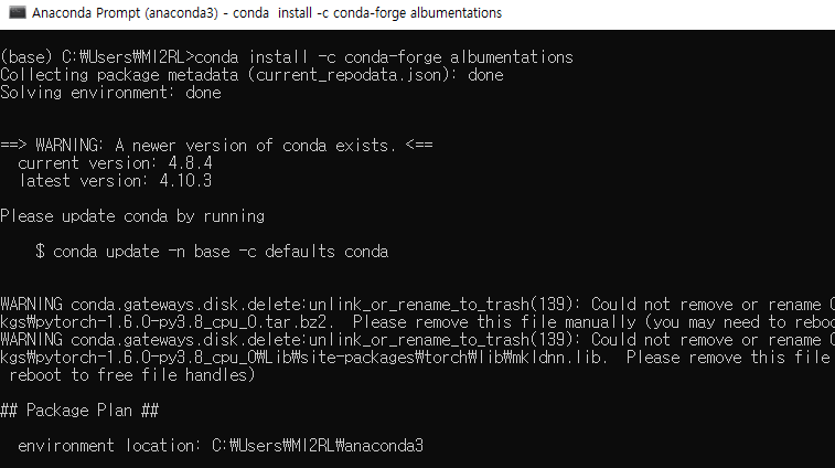
필자는 현재 Visual Studio Code IDE (=VS Code)를 이용해 코딩을 하고 있는데, VS Code의 interpreter가 아나콘다(anaconda) 가상환경에 연동되어 있기 때문에, Albumentations 패키지를 설치하기 위해서 anaconda 명령어를 이용하도록 하겠습니다.

(↓↓↓아나콘다 가상환경 설명↓↓↓)

https://89douner.tistory.com/73?category=878197 

(↓↓↓아나콘다 가상환경과 VS code interpreter 연동방법↓↓↓)

https://89douner.tistory.com/74

1. Albumentations 패키지 설치하기

앞서 필자는 VS code interpereter에 아나콘다 가상환경을 연동해서 사용하기 때문에, anaconda 명령어를 통해 albumentations 패키지를 설치할 것이라고 언급했습니다. 

Anaconda 명령어를 이용해 albumentations 패키지를 설치하는 방식은 아래사이트에서 확인할 수 있습니다.

https://anaconda.org/conda-forge/albumentations

(↓↓↓ albumentations 설치 명령어 ↓↓↓)

conda install -c conda-forge albumentations

anaconda prompt를 열고 위와 같이 설치 명령어를 입력한 후 설치를 진행해줍니다.

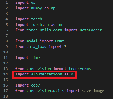
설치가 완료되면 아래와 같이 자신이 코드를 작성하고 있는 디렉토리에서 albumentations 모듈을 import해 관련 attribute or function들을 사용하면 됩니다. 그럼 지금부터 albumentations 모듈을 사용하여 데이터 로드 하는 방식을 설명해보도록 하겠습니다.

2. Albumentation 데이터 로드 코드

지금부터 설명하는 내용은 대부분 이전글 ("1-1. Data Load (Feat. torchvision transform) 을 기반으로 달라진 부분들에 대해서만 설명하도록 하겠습니다. 다시 말해, albumentation 을 이용하여 데이터 로드를 할 때 torchvision transform 기반으로 데이터 로드를 하는 코드들 중 어느 부분을 수정하면 되는지 말씀드리겠습니다. (그러므로 이전 글을 읽어보시는걸 추천합니다)

(↓↓↓ 이전 글: torchvision.transform 기반 데이터 로드 방식↓↓↓)

https://89douner.tistory.com/299?category=1001221 

먼저, 필자는 "alb_data_load.py, alb_train2.py"와 같이 파이썬 파일을 만들었습니다.

이 파일의 코드는 이전 글에서 설명한 코드들을 복사 붙여넣기 하여, albumentation을 적용하기 위해 수정된 최종 코드입니다.

[alb_data_laod.py]

import os
import numpy as np
import glob

import torch
import torch.nn as nn


## 데이터 로더를 구현하기
class Dataset(torch.utils.data.Dataset):
    def __init__(self, data_dir, transform=None):
        self.data_dir = data_dir
        self.transform = transform

        self.data_dir_input = self.data_dir + '/input'
        self.data_dir_label = self.data_dir + '/label'

        lst_data_input = os.listdir(self.data_dir_input)
        lst_data_label = os.listdir(self.data_dir_label)

        self.lst_label = lst_data_label
        self.lst_input = lst_data_input

    def __len__(self):
        return len(self.lst_label)

    def __getitem__(self, index):
        label = np.load(os.path.join(self.data_dir_label, self.lst_label[index]))
        input = np.load(os.path.join(self.data_dir_input, self.lst_input[index]))

        if label.ndim == 2:
            label = label[:, :, np.newaxis]
        if input.ndim == 2:
            input = input[:, :, np.newaxis]

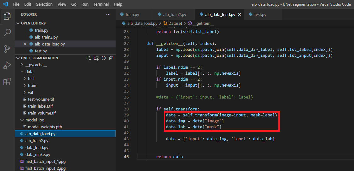
        #data = {'input': input, 'label': label}

        if self.transform:
            data = self.transform(image=input, mask=label)
            data_img = data["image"]
            data_lab = data["mask"]

            data = {'input': data_img, 'label': data_lab}
            

        return data

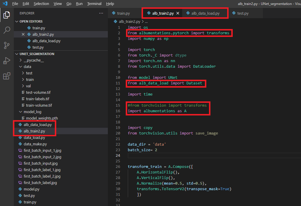
[alb_train2.py]

import os
from albumentations.pytorch import transforms
import numpy as np

import torch
from torch._C import dtype
import torch.nn as nn
from torch.utils.data import DataLoader

from model import UNet
from alb_data_load import Dataset

import time

#from torchvision import transforms
import albumentations as A


import copy
from torchvision.utils import save_image

data_dir = 'data'
batch_size= 2


transform_train = A.Compose([
    A.HorizontalFlip(),
    A.VerticalFlip(), 
    A.Normalize(mean=0.5, std=0.5),
    transforms.ToTensorV2(transpose_mask=True)
    ])


transform_val = A.Compose([
    A.HorizontalFlip(), 
    A.Normalize(mean=0.5, std=0.5),
    transforms.ToTensorV2(transpose_mask=True)
    ])


dataset_train = Dataset(data_dir=os.path.join(data_dir, 'train'), transform=transform_train)
loader_train = DataLoader(dataset_train, batch_size=batch_size, shuffle=False, num_workers=0)

dataset_val = Dataset(data_dir=os.path.join(data_dir, 'val'), transform=transform_val)
loader_val = DataLoader(dataset_val, batch_size=batch_size, shuffle=False, num_workers=0)


# 그밖에 부수적인 variables 설정하기
num_data_train = len(dataset_train)
num_data_val = len(dataset_val)

num_batch_train = np.ceil(num_data_train / batch_size)
num_batch_val = np.ceil(num_data_val / batch_size)

device = torch.device("cuda:0" if torch.cuda.is_available() else "cpu")

## 네트워크 생성하기
net = UNet().to(device)

## 손실함수 정의하기
fn_loss = nn.BCEWithLogitsLoss().to(device)

## Optimizer 설정하기
optim = torch.optim.Adam(net.parameters(), lr=1e-3)

## 네트워크 학습시키기
st_epoch = 0
num_epoch = 30
# TRAIN MODE

def train_model(net, fn_loss, optim, num_epoch):
    since = time.time()

    best_model_wts = copy.deepcopy(net.state_dict())
    best_loss = 100

    for epoch in range(st_epoch + 1, num_epoch + 1):
        net.train()
        loss_arr = []

        for batch, data in enumerate(loader_train, 1):
            data['label'] = data['label']/255.0

            input = data['input']
            label = data['label']

            # forward pass
            label = data['label'].to(device)
            input = data['input'].to(device)

            output = net(input)

            # backward pass
            optim.zero_grad()

            loss = fn_loss(output, label)
            loss.backward()

            optim.step()

            # 손실함수 계산
            loss_arr += [loss.item()]

            print("TRAIN: EPOCH %04d / %04d | BATCH %04d / %04d | LOSS %.4f" %
                (epoch, num_epoch, batch, num_batch_train, np.mean(loss_arr)))


        with torch.no_grad():
            net.eval()
            loss_arr = []

            for batch, data in enumerate(loader_val, 1):
                data['label'] = data['label']/255.0

                # forward pass
                label = data['label'].to(device, dtype=torch.float32)
                input = data['input'].to(device, dtype=torch.float32)

                output = net(input)

                # 손실함수 계산하기
                loss = fn_loss(output, label)

                loss_arr += [loss.item()]

                print("VALID: EPOCH %04d / %04d | BATCH %04d / %04d | LOSS %.4f" %
                        (epoch, num_epoch, batch, num_batch_val, np.mean(loss_arr))) 

            epoch_loss = np.mean(loss_arr)

            # deep copy the model
            if epoch_loss < best_loss:
                best_loss = epoch_loss
                best_model_wts = copy.deepcopy(net.state_dict())

        print()
    
    time_elapsed = time.time() - since
    print('Training complete in {:.0f}m {:.0f}s'.format(
        time_elapsed // 60, time_elapsed % 60))
    print('Best val loss: {:4f}'.format(best_loss))

    # load best model weights
    net.load_state_dict(best_model_wts)
    return net

model_ft = train_model(net, fn_loss, optim, num_epoch)
torch.save(model_ft.state_dict(), './model_log/model_weights.pth')

그럼 위의 코드와 이전 글의 코드를 비교하면서 설명을 해보도록 하겠습니다.

3. Import

먼저 이전 글에서 추가할 import 부분에 대해서 설명하겠습니다.

1. alb_data_load.py 라는 새로운 데이터 로드 파일을 만들어 주었으므로 alb_data_load의 Dataset을 import 합니다.
   • from alb_data_load import Dataset
2. 설치한 albumentaion 관련 모듈을 import 해줍니다.
   • import albumentations as A
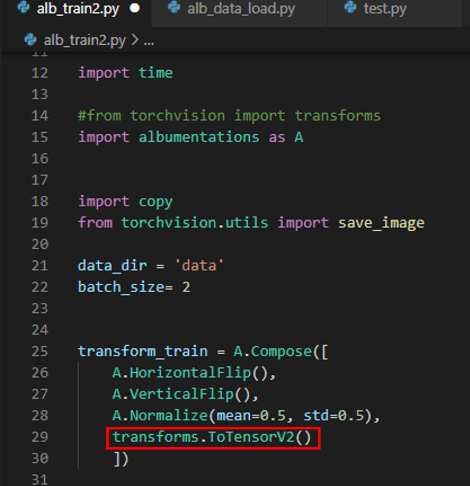
   • from albumentations.pytorch import transfroms → 아래 "그림3"에서 transfor_train 부분을 보면 마지막에 ToTensorV2가 구현된 것을 볼 수 있습니다. ToTensorV2만 "albumentations.pytorch"로부터 import 한다는 걸 인지하세요!

4. alb_data_load.py 변경

4-1. albumentation.transform(image, mask)

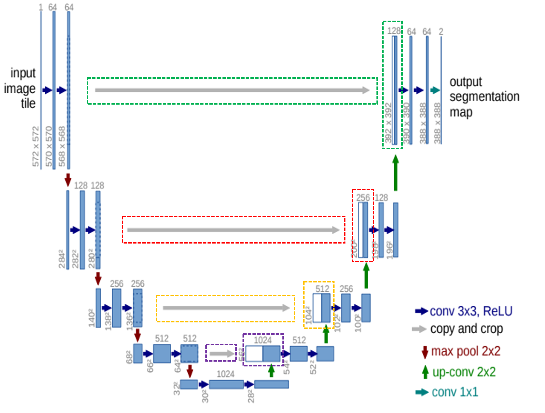
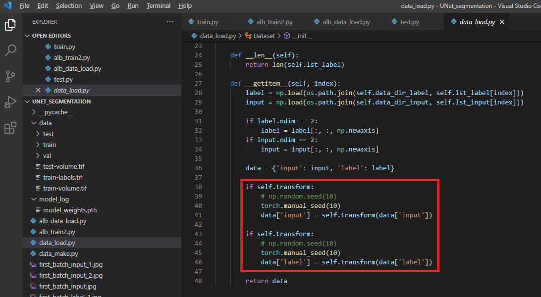
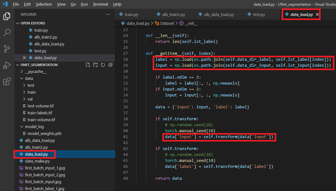
먼저, 이전 글에서 설명한 torchvision.transform의 인자형태를 보도록 하겠습니다. (아래 "4그림")

transform(data['input']), transform(data['label']) 이렇게 transform에는 하나의 리스트 인자(argument)만 받을 수 있게 되어 있습니다 (이러한 부분 때문에 torch.manual_seed()를 사용했죠 ← 자세한 설명은 이전 글 참고!)

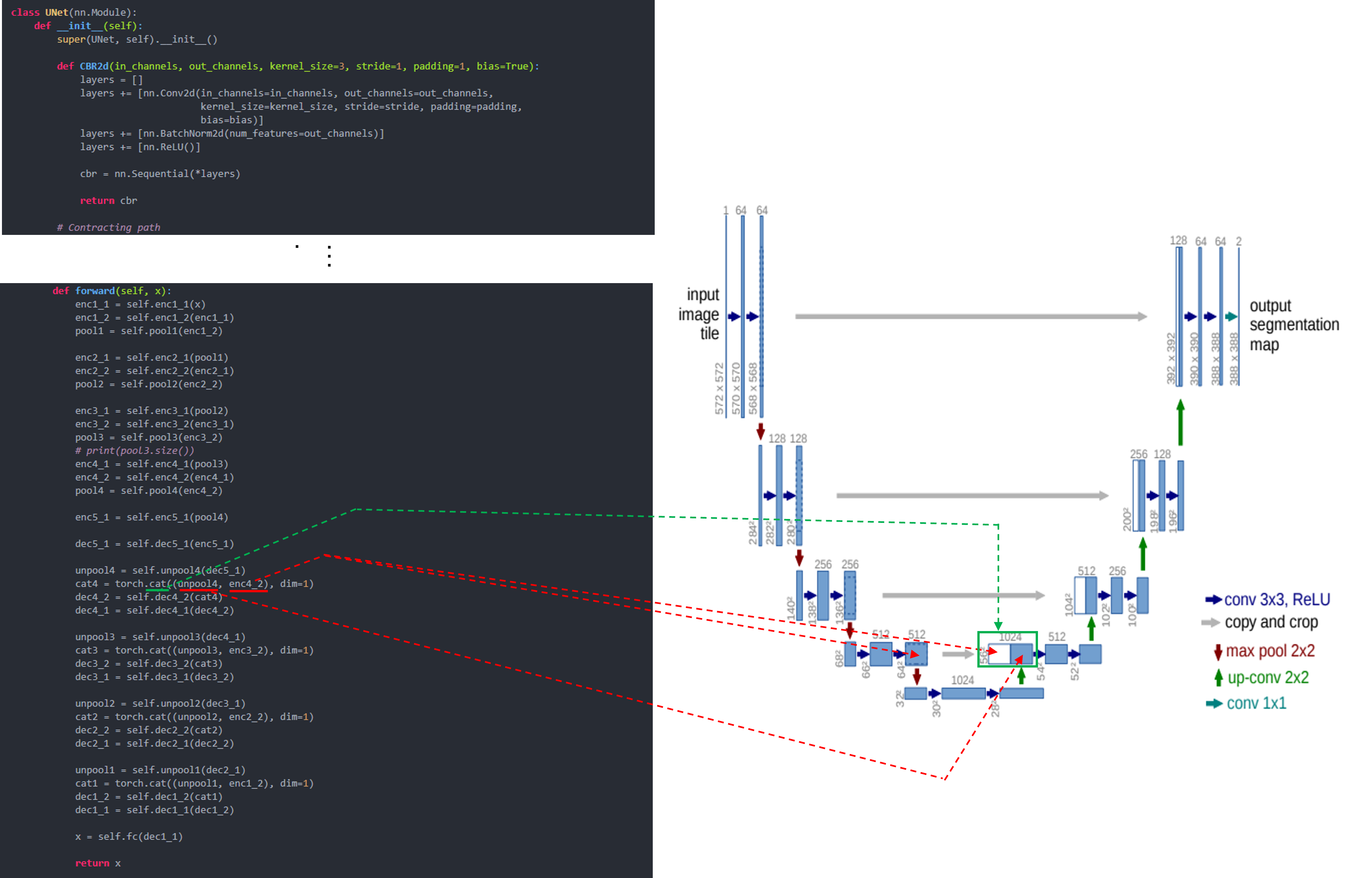
그렇다면, albumentation에서 제공해주는 transform을 이용하면 위의 부분(="그림4"의 빨간색 박스)이 어떻게 바뀔 수 있을까요?

albumentation에서 제공해주는 transform은 두 개의 리스트 인자를 받을 수 있게 되어 있습니다. (아래 "그림5")

그래서 training image, training label을 동시에 넘겨줄 수 있기 때문에 따로 seed를 고정시켜줄 필요가 없습니다. (실제로 data_img, data_lab 데이터를 10번 정도 이미지화해서 살펴봐도 augmentation이 동일하게(일치하게) 적용되는 것을 확인할 수 있었습니다)

5. alb_train2.py 변경

5-1. transform.Compose → A.Compose

(이전 글에서 봤듯이) transform.Compose에 구현된 augmentation을 적용하기 위해 입력되는 데이터 형식은 numpy입니다. 

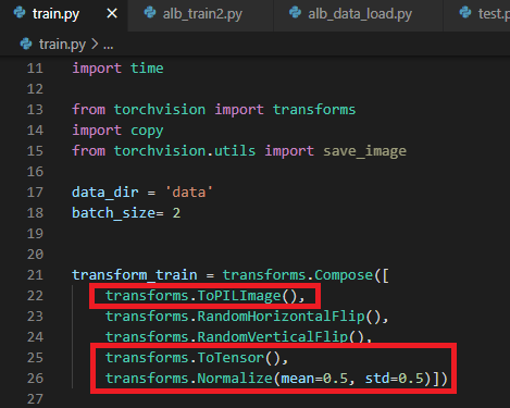
먼저, 이전 글에서 사용했던 torchvision.transform.Compose에 구현된 순서를 살펴보겠습니다. (아래 "그림8")

torchvision.transform.Compose에서 제공하는 augmentation (ex: RandomHorizontalFlip(), etc..) 을 적용하기 위해서는 PIL 타입의 데이터가 입력되어야 합니다. 그래서 아래와 같이 "transforms.ToPILImage()" 를 먼저 수행시켜주어야 합니다. 그리고, PIL 타입을 torch tensor 타입으로 변경시켜준 후 (by "ToTensor()"), Normalize() 작업을 진행해줍니다.

그렇다면, albumentation.transform.Compose에서는 어떤 순서로 구성되는지 알아볼까요? (아래 "그림9")

우선 numpy 형식으로 입력되는 데이터를 PIL 형식으로 변경해줄 필요가 없기 때문에 "ToPILImage()"를 사용할 필요가 없습니다. 그리고, torch tensor 형태로 변경하기 전에 먼저 Normalize를 적용해주네요. 그리고, ToTensorV2를 적용해줍니다.

여기서 좀 더 보충해서 설명해야할 부분이 Normalize(), ToTensorV2() 입니다.

5-2. Normalize()

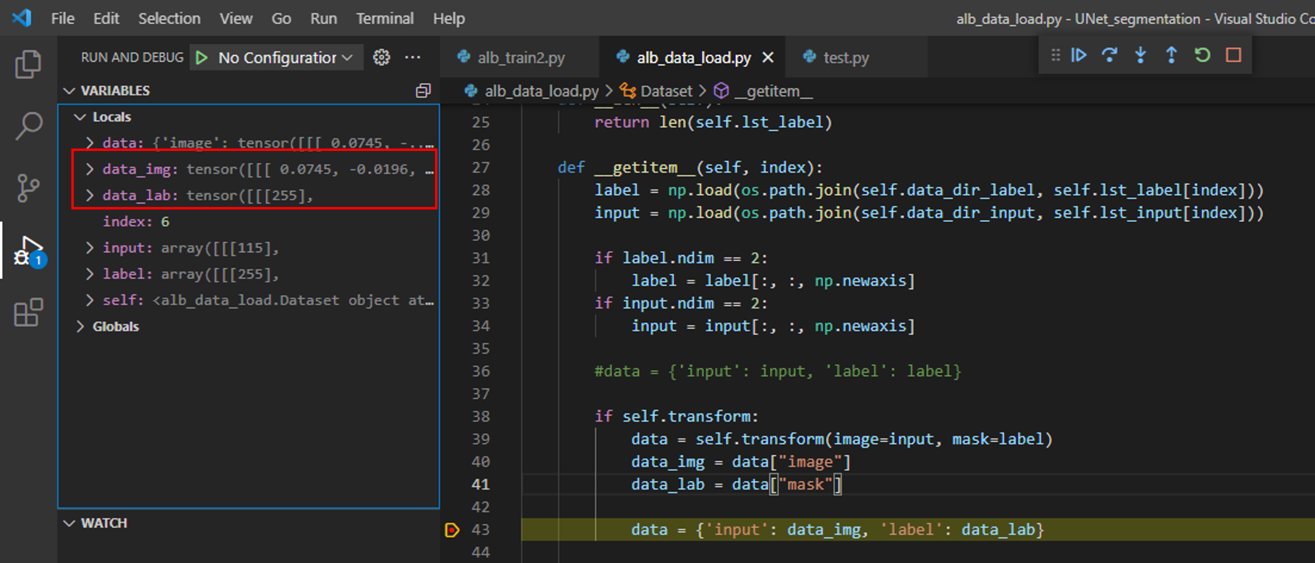
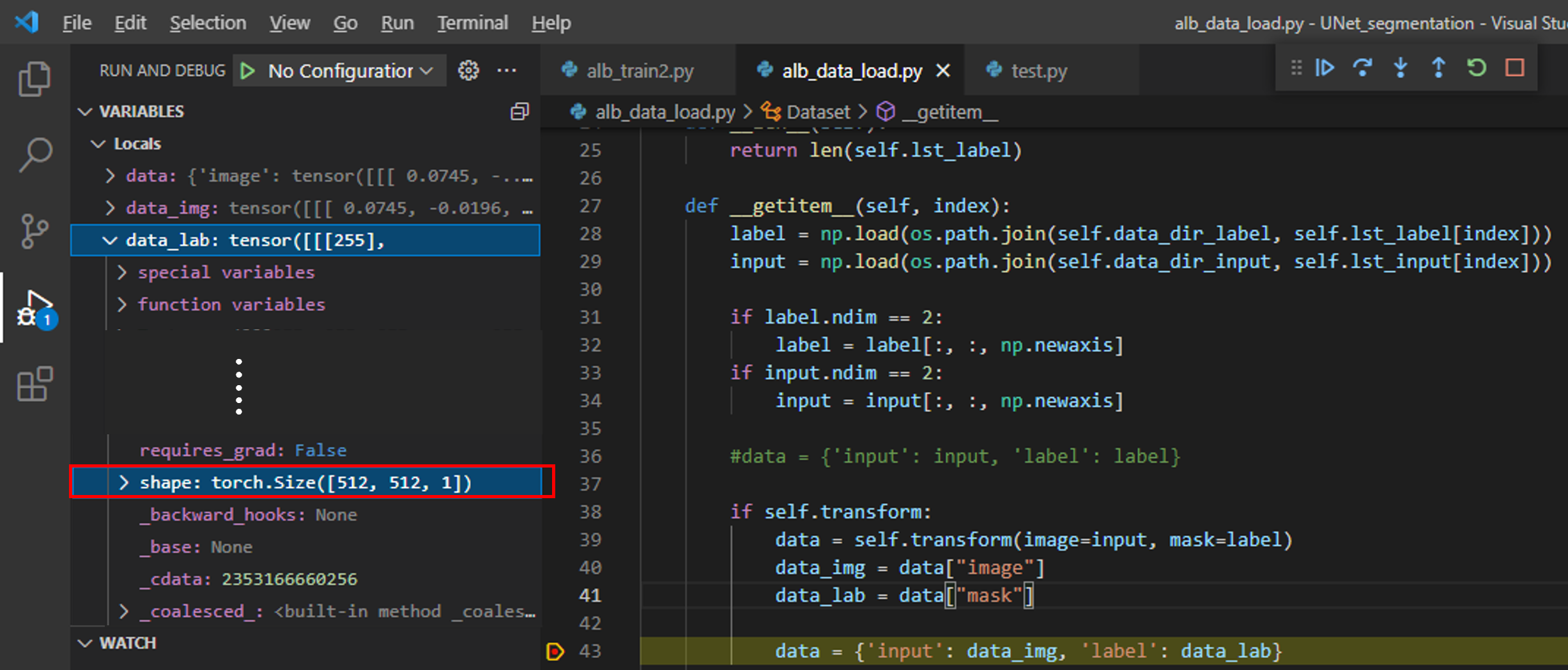
먼저, 아래 "그림10"처럼 breakpoint를 걸어주고 "alb_train2.py"를 실행시켜봅시다.

위 "그림10"처럼 디버깅을 하면 data_img, data_lab 값을 살펴볼 수 있습니다. 

그런데, data_img에는 Normalize가 적용이 안되어 있습니다.

이러한 사실로 볼때 albumentation.transform.Compose에 적용되는 augmentation 중에 Normalize()는 label(=mask)에 적용되지 않는 듯합니다.

5-3. ToTensorV2()

이전 글에서 torchvision.transform.ToTensor()는 아래와 같은 기능을 한다고 했습니다.

• Converts a PIL Image or numpy.ndarray (H x W x C) in the range [0, 255] to a torch.FloatTensor of shape (C x H x W) in the range [0.0, 1.0] if the PIL Image belongs to one of the modes (L, LA, P, I, F, RGB, YCbCr, RGBA, CMYK, 1) or if the numpy.ndarray has dtype = np.uint8

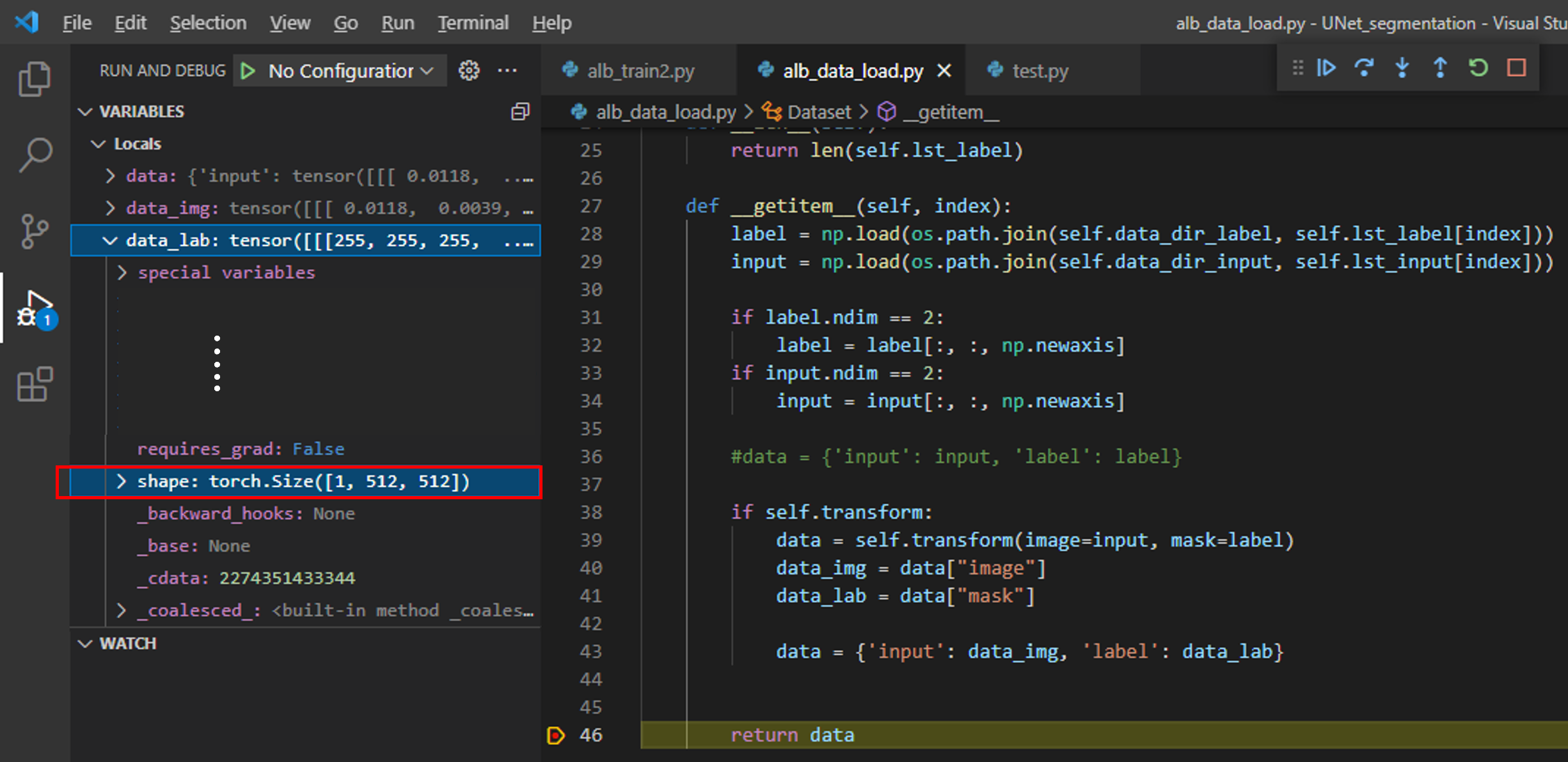
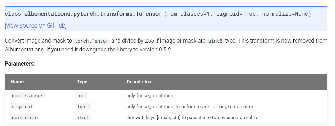
그런데, albumentation.transform.ToTensorV2() 결과 label의 타입이 numpy (=H x W x C) 에서 torch tensor 타입 (=C x H x W)으로 바뀌었지만, range는 그대로 0~255인 것을 확인할 수 있습니다.  (아래 "그림11")

그 이유를 아래 "albumentations.pytorch.transforms.ToTensorV2()" API를 살펴본 후 알 수 있었습니다.

https://albumentations.ai/docs/api_reference/pytorch/transforms/

쉽게 말해 albumentation 패키지 version 0.5.2 이후 부터는 255로 나누어주어 range를 0~1로 변경해주는 기능이 제거된다. 이러한 사실통해 살펴 볼때, 앞서 "data_img" 값들이 0~1로 범위가 변경된 이유는 Normalize()에 해당 기능(← 값의 범위를 0~1로 변경해주는 기능)이 들어있기 때문인듯 합니다. (앞서 albumentation.transforms.Normalize()는 label이 아닌 image에만 적용된다고 언급했습니다)

하지만, label(=mask)에 해당하는 값이 loss function(=crossentropy)의 인자 값으로 들어가기 위해서는 label이 0 or 1의 값을 갖아야 합니다. 즉, label 데이터 값의 255를 1로 변경해주어야 하는 것이죠 (or labeling smoothing을 적용하려면 label의 값의 범위가 0~1 사이로 변경되어야겠죠?)

이 부분은 간단하게 구현해줄 수 있습니다.

그냥 "alb_train2.py"에서 아래와 같이 data['label']을 255로 나누어주면 됩니다.

[주의사항]

아래와 같이 "ToTensorV2()"에 transpose_mask 부분을 명시해주지 않으면 False 값이 default가 됩니다.

위와 같이 코드를 실행 시키면 torch tensor 형식(=C x H x W)이 아닌  (H x W x C) 형식인걸 알 수 있습니다.

물론 (H x W x C) 구조를 permute()을 이용해 쉽게  (C x H x W) 구조로 변경 가능하지만, 그냥 ToTensorV2(transpose_mask=True)를 해주면 자동으로 구조변경이 된다는 점을 알아두시면 좋을 듯 합니다.

(↓↓↓permute() 사용법 ↓↓↓)

https://devbruce.github.io/machinelearning/ml-05-np_torch_summary/

6. albumentation 응용

albumentation.transform.Compose 내부에 적용되는 augmetation 조합은 굉장히 다양하게 가져갈 수 있습니다.

방법은 아래 사이트의 "albumentations 응용 사례" 부분을 참고해주세요!

https://hoya012.github.io/blog/albumentation_tutorial/

지금까지 albumentations 패키지를 이용한 segmentation 데이터 로드 코드를 알아보았습니다.

감사합니다.

안녕하세요.

이번 글에서는 "UNet (딥러닝 segmentation모델)" 학습을 위해 해당 모델에 입력으로 들어갈 데이터들이 어떤 과정을 통해 load 되는지 알아보도록 하겠습니다. 

코드는 아래 사이트를 기반으로 수정하였으니 아래 영상을 먼저 참고하시면 글을 이해하시는데 도움이 될 것으로 생각됩니다.

https://www.youtube.com/watch?v=1gMnChpUS9k 

위의 강의에서는 augmentation 부분을 직접구현해주었는데, 이번 글에서는 torchvision에서 augmentation을 위해 제공해주는 torchvision.transform 모듈을 적용하여 data load 하는 내용을 설명하려고 합니다.

[data_load.py]

import os
import numpy as np
import glob

import torch
import torch.nn as nn


## 데이터 로더를 구현하기
class Dataset(torch.utils.data.Dataset):
    def __init__(self, data_dir, transform=None, seed=None):
        self.data_dir = data_dir
        self.transform = transform
        self.seed = seed

        self.data_dir_input = self.data_dir + '/input'
        self.data_dir_label = self.data_dir + '/label'

        lst_data_input = os.listdir(self.data_dir_input)
        lst_data_label = os.listdir(self.data_dir_label)

        self.lst_label = lst_data_label
        self.lst_input = lst_data_input

    def __len__(self):
        return len(self.lst_label)

    def __getitem__(self, index):
        label = np.load(os.path.join(self.data_dir_label, self.lst_label[index]))
        input = np.load(os.path.join(self.data_dir_input, self.lst_input[index]))

        if label.ndim == 2:
            label = label[:, :, np.newaxis]
        if input.ndim == 2:
            input = input[:, :, np.newaxis]

        data = {'input': input, 'label': label}

        if self.transform: 
            torch.manual_seed(self.seed)
            data['input'] = self.transform(data['input'])
            
        if self.transform:   
            torch.manual_seed(self.seed)
            data['label'] = self.transform(data['label'])

        return data

[train.py]

import os
import numpy as np

import torch
import torch.nn as nn
from torch.utils.data import DataLoader

from model import UNet
from data_load import *

import time

from torchvision import transforms
import copy
from torchvision.utils import save_image

data_dir = 'data'
batch_size= 2
data_load_seed = 10

transform_train = transforms.Compose([
    transforms.ToPILImage(), 
    transforms.RandomHorizontalFlip(),
    transforms.RandomVerticalFlip(), 
    transforms.ToTensor(),
    transforms.Normalize(mean=0.5, std=0.5)])


transform_val = transforms.Compose([
    transforms.ToPILImage(), 
    transforms.RandomHorizontalFlip(), 
    transforms.ToTensor(),
    transforms.Normalize(mean=0.5, std=0.5)
    ])


dataset_train = Dataset(data_dir=os.path.join(data_dir, 'train'), transform=transform_train, seed=data_load_seed)
loader_train = DataLoader(dataset_train, batch_size=batch_size, shuffle=False, num_workers=0)

dataset_val = Dataset(data_dir=os.path.join(data_dir, 'val'), transform=transform_val, seed=data_load_seed)
loader_val = DataLoader(dataset_val, batch_size=batch_size, shuffle=False, num_workers=0)


# 그밖에 부수적인 variables 설정하기
num_data_train = len(dataset_train)
num_data_val = len(dataset_val)

num_batch_train = np.ceil(num_data_train / batch_size)
num_batch_val = np.ceil(num_data_val / batch_size)

device = torch.device("cuda:0" if torch.cuda.is_available() else "cpu")

## 네트워크 생성하기
net = UNet().to(device)

## 손실함수 정의하기
fn_loss = nn.BCEWithLogitsLoss().to(device)

## Optimizer 설정하기
optim = torch.optim.Adam(net.parameters(), lr=1e-3)

## 네트워크 학습시키기
st_epoch = 0
num_epoch = 30
# TRAIN MODE

def train_model(net, fn_loss, optim, num_epoch):
    since = time.time()

    best_model_wts = copy.deepcopy(net.state_dict())
    best_loss = 100

    for epoch in range(st_epoch + 1, num_epoch + 1):
        net.train()
        loss_arr = []

        for batch, data in enumerate(loader_train, 1):
            data['label'] = data['label']*0.5+0.5 #denormalization -> X*std+mean
            label = data['label']
            input = data['input']

            # first_batch_input = input[0]*0.5+0.5
            # save_image(first_batch_input, 'first_batch_input.jpg')

            # first_batch_label = label[0]
            # save_image(first_batch_label, 'first_batch_label.jpg')

            # forward pass
            label = data['label'].to(device)
            input = data['input'].to(device)

            output = net(input)

            # backward pass
            optim.zero_grad()

            loss = fn_loss(output, label)
            loss.backward()

            optim.step()

            # 손실함수 계산
            loss_arr += [loss.item()]

            print("TRAIN: EPOCH %04d / %04d | BATCH %04d / %04d | LOSS %.4f" %
                (epoch, num_epoch, batch, num_batch_train, np.mean(loss_arr)))


        with torch.no_grad():
            net.eval()
            loss_arr = []

            for batch, data in enumerate(loader_val, 1):
                data['label'] = data['label']*0.5+0.5 #denormalization -> X*std+mean

                # forward pass
                label = data['label'].to(device)
                input = data['input'].to(device)

                output = net(input)

                # 손실함수 계산하기
                loss = fn_loss(output, label)

                loss_arr += [loss.item()]

                print("VALID: EPOCH %04d / %04d | BATCH %04d / %04d | LOSS %.4f" %
                        (epoch, num_epoch, batch, num_batch_val, np.mean(loss_arr))) 

            epoch_loss = np.mean(loss_arr)

            # deep copy the model
            if epoch_loss < best_loss:
                best_loss = epoch_loss
                best_model_wts = copy.deepcopy(net.state_dict())

        print()
    
    time_elapsed = time.time() - since
    print('Training complete in {:.0f}m {:.0f}s'.format(
        time_elapsed // 60, time_elapsed % 60))
    print('Best val loss: {:4f}'.format(best_loss))

    # load best model weights
    net.load_state_dict(best_model_wts)
    return net

model_ft = train_model(net, fn_loss, optim, num_epoch)
torch.save(model_ft.state_dict(), './model_log/model_weights.pth')

위에 있는 코드들 중에서 핵심적인 코드 또는 수정한 코드에 대해서만 설명 하도록 하겠습니다 (좀 더 구체적인 설명을 듣고 싶으신 분은 위에 링크를 걸어둔 유튜브 강의를 참고해주시면 감사하겠습니다)

0.Dataset 클래스

from torchvision import transforms

transform_train = transforms.Compose([
    transforms.ToPILImage(), 
    transforms.RandomHorizontalFlip(),
    transforms.RandomVerticalFlip(), 
    transforms.ToTensor(),
    transforms.Normalize(mean=0.5, std=0.5)])
    
dataset_train = Dataset(data_dir=os.path.join(data_dir, 'train'), transform=transform_train)
loader_train = DataLoader(dataset_train, batch_size=batch_size, shuffle=True, num_workers=0)

Dataset()에 넘겨주는 인자를 보면 두 가지 입니다.

1. train 디렉토리
2. 적용할 augmentation 기법들 → transform

그럼 Dataset에 구현되있는 부분 중에 train 디렉토리에 해당하는 부분들을 살펴보도록 하겠습니다.

1. train 디렉토리와 관련된 부분

## 데이터 로더를 구현하기
class Dataset(torch.utils.data.Dataset):
    def __init__(self, data_dir, transform=None):
        self.data_dir = data_dir
        self.transform = transform

        self.data_dir_input = self.data_dir + '/input'
        self.data_dir_label = self.data_dir + '/label'

        lst_data_input = os.listdir(self.data_dir_input)
        lst_data_label = os.listdir(self.data_dir_label)

        self.lst_label = lst_data_label
        self.lst_input = lst_data_input

    def __len__(self):
        return len(self.lst_label)

    def __getitem__(self, index):
        label = np.load(os.path.join(self.data_dir_label, self.lst_label[index]))
        input = np.load(os.path.join(self.data_dir_input, self.lst_input[index]))

        if label.ndim == 2:
            label = label[:, :, np.newaxis]
        if input.ndim == 2:
            input = input[:, :, np.newaxis]

        data = {'input': input, 'label': label}

위의 코드를 살펴보면 train 디렉토리가 Dataset의 인자로 넘어가게 되면 아래 그림1에 있는 디렉토리의 numpy 데이터에 접근한다는 것을 확인할 수 있습니다.

실제로 breakpiont를 통해 살펴보면 input, label 이라는 변수에 모든 numpy 데이터들이 리스트 형태로 저장되는 것을 확인할 수 있습니다.

앞선 글에서 저장된 데이터의 형태가 (H,W) 임을 확인할 수 있었습니다.

또한, 딥러닝 모델의 학습을 위해서 (H,W)의 2차원 구조가 (H,W,C)의 3차원 구조로 변경되어야 한다고도 말씀드렸습니다.

(↓↓↓ 아래 글에서 "2-3) numpy 형태로 저장하는 이유" 부분을 참고해주세요↓↓↓)

https://89douner.tistory.com/298?category=1001221 

(아래 "그림3"처럼 shape 부분을 살펴보면 label, input 변수에 저장된 데이터는 numpy형식의2차원 데이터입니다.)

위와 같은 2차원 구조를 3차원으로 늘려주기 위해 아래 코드가 실행됩니다.

[data_load.py]

        if label.ndim == 2:
            label = label[:, :, np.newaxis]
        if input.ndim == 2:
            input = input[:, :, np.newaxis]

2. torchvision.transform 

앞서 설명드린 내용은 아래 코드에서 'if self.transform' 직전까지 부분입니다.

## 데이터 로더를 구현하기
class Dataset(torch.utils.data.Dataset):
    def __init__(self, data_dir, transform=None):
        self.data_dir = data_dir
        self.transform = transform

        self.data_dir_input = self.data_dir + '/input'
        self.data_dir_label = self.data_dir + '/label'

        lst_data_input = os.listdir(self.data_dir_input)
        lst_data_label = os.listdir(self.data_dir_label)

        self.lst_label = lst_data_label
        self.lst_input = lst_data_input

    def __len__(self):
        return len(self.lst_label)

    def __getitem__(self, index):
        label = np.load(os.path.join(self.data_dir_label, self.lst_label[index]))
        input = np.load(os.path.join(self.data_dir_input, self.lst_input[index]))

        if label.ndim == 2:
            label = label[:, :, np.newaxis]
        if input.ndim == 2:
            input = input[:, :, np.newaxis]

        data = {'input': input, 'label': label}

        if self.transform:
            torch.manual_seed(10)
            data['input'] = self.transform(data['input'])
            
        if self.transform: 
            torch.manual_seed(10)
            data['label'] = self.transform(data['label'])

        return data

그렇다면, 지금부터는 self.transform 과 관련된 내용에 대해서 설명하도록 하겠습니다.

self.transform 부분은 Dataset 클래스에서 두 번째로 살펴볼 인자인 transform과 관련이 있습니다.

(transform은 torchvision에서 제공해주는 모듈로 사용하고 있습니다.)

from torchvision import transforms

transform_train = transforms.Compose([
    transforms.ToPILImage(), 
    transforms.RandomHorizontalFlip(),
    transforms.RandomVerticalFlip(), 
    transforms.ToTensor(),
    transforms.Normalize(mean=0.5, std=0.5)])
    
dataset_train = Dataset(data_dir=os.path.join(data_dir, 'train'), transform=transform_train)
loader_train = DataLoader(dataset_train, batch_size=batch_size, shuffle=True, num_workers=0)

2-1) transforms.ToPILImage()

우선 위의 코드에서 transforms.Compose 부분을 살펴보겠습니다.

현재 아래코드가 실행되기 직전의 data['input']에 들어 있는 데이터 구조는 3차원 (H,W,C) 형태로 변경된 numpy 데이터 입니다.

        if self.transform:
            torch.manual_seed(10)
            data['input'] = self.transform(data['input'])

그리고, self.transform(data['input'])이 실행되면 transform.Compose에 적힌 순서대로 데이터의 변화가 일어납니다.

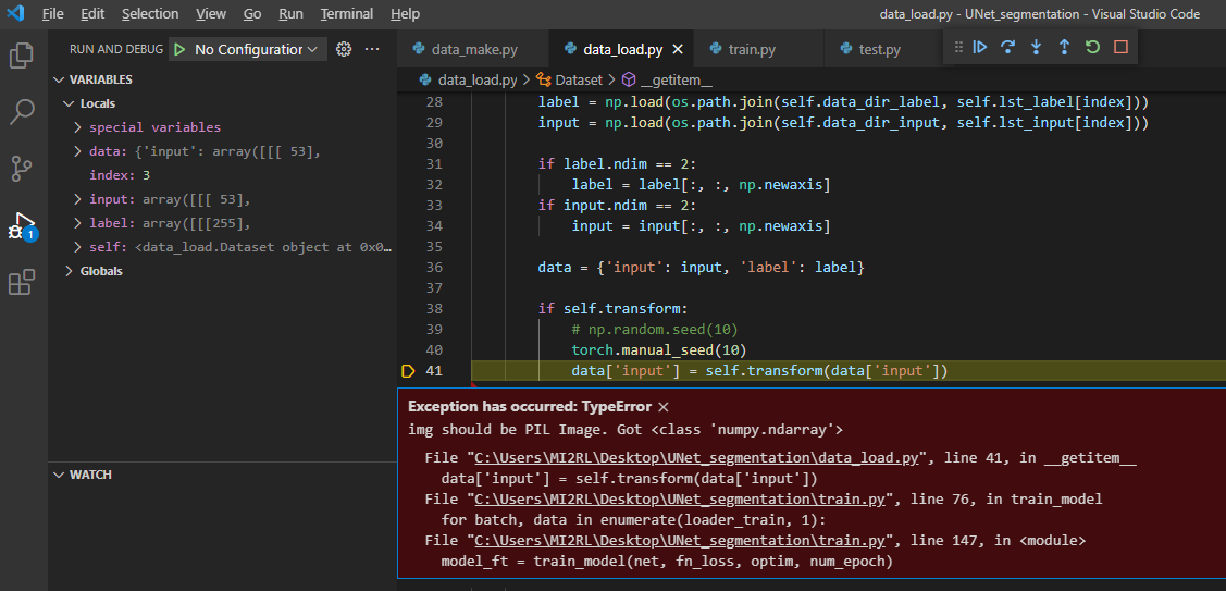
먼저, RandomHorizontalFlip과 같이 torchvision에서 제공해주는 augmentation 기법을 사용하기 위해서는 현재 numpy 형식의 데이터가 PIL 이미지 형식의 데이터가 입력값으로 들어와야 합니다.

그렇기 때문에 transform.Compose 부분에서 제일 처음으로 "transforms.ToPILImage()"를 작성해줍니다. 

[주의사항1]

만약, ToPILImage() 부분을 작성하지 않으면 아래와 같은 에러가 발생합니다.

에러 메시지 내용은 아래와 같습니다.

"현재 입력 받은 이미지의 형식은 numpy.ndarray 이니까 (="Got <class 'numpy.ndarray'>),  PIL 형태로 바꿔주어야 합니다(="img should be PIL Image")"

2-2) transforms.ToTensor, transforms.Normalize 위치

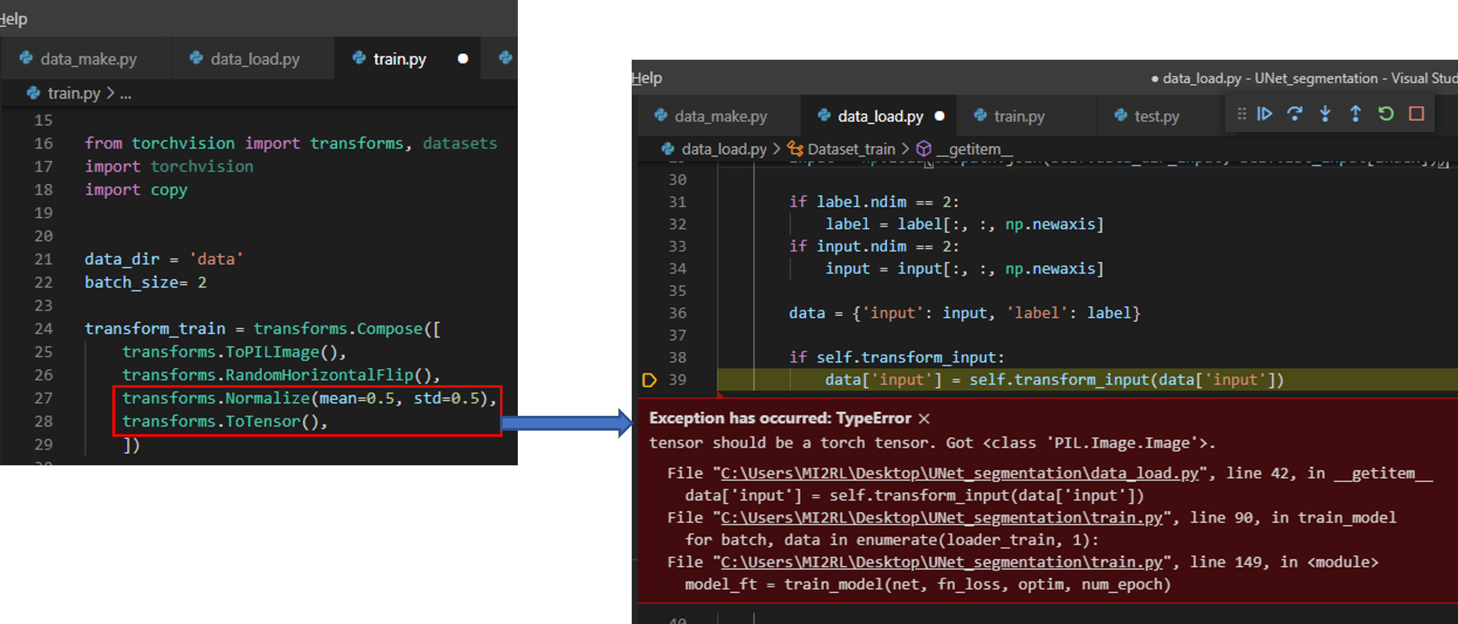
Pytorch에서 제공해주는 transforms.Normalize()를 사용하려면 항상 transforms.ToTensor() 이후에 위치해야 합니다.  

이렇게 위치시켜야하는 이유는 Normalize()가 torch tensor 형식을 입력으로 받기 때문입니다.

아래 코드를 기반으로 설명하면, RandomVerticalFlip까지 적용된 데이터 형식은 PIL image 형식 (512x 512x 1) 인데, 이것을 Normalize가 적용되려면 (1x 512x 512) 형식으로 변경되어야 합니다 (pixel range도 0~1로 변경되어야 합니다).   

• ToTensor(): Converts a PIL Image or numpy.ndarray (H x W x C) in the range [0, 255] to a torch.FloatTensor of shape (C x H x W) in the range [0.0, 1.0]

from torchvision import transforms

transform_train = transforms.Compose([
    transforms.ToPILImage(), 
    transforms.RandomHorizontalFlip(),
    transforms.RandomVerticalFlip(), 
    transforms.ToTensor(),
    transforms.Normalize(mean=0.5, std=0.5)])
    
dataset_train = Dataset(data_dir=os.path.join(data_dir, 'train'), transform=transform_train)
loader_train = DataLoader(dataset_train, batch_size=batch_size, shuffle=True, num_workers=0)

[주의사항2]

만약, 순서를 아래와 같이 위치시켰다면 에러 메시지가 출력됩니다.

• transforms.Normalize
• transforms.ToTensor

에러 메시지의 내용은 다음과 같습니다.

"현재 입력 받은 이미지의 형식은 PIL기반 tensor이니까 (="Got <class 'PIL.Image.Image'>),  PIL 형태로 바꿔주어야 합니다(="tensor should be a torch tensor")"

2-3. input, label에 적용되는 transform seed 고정해주기

아래 코드를 살펴보면 "torch.manual_seed(10)"이라는 것이 있습니다.

[data_load.py]

        if self.transform:  
            torch.manual_seed(10)
            data['input'] = self.transform(data['input'])
            
        if self.transform:
            torch.manual_seed(10)
            data['label'] = self.transform(data['label'])

"torch.manual_seed(10)" 코드를 추가하는 이유를 설명하기 위해, "torch.manual_seed(10)"가 없을 때 일어나는 일에 대해서 알아보도록 하겠습니다.

우선 "data_load.py" 부분에서 "torch.manual_seed(10)" 코드를 주석 처리해보겠습니다.

        if self.transform:  
            #torch.manual_seed(10)
            data['input'] = self.transform(data['input'])
            
        if self.transform:
            #torch.manual_seed(10)
            data['label'] = self.transform(data['label'])

그리고, "train.py" 부분에서 딥러닝 모델에 입력되기 직전의 이미지 상태를 알아보도록 하겠습니다.

이전 transforms.Compose에서 input, label에 모두 transforms.Normalize가 적용이 됐다는걸 알 수 있습니다.

그런데, 생각해보면 label에는 Normalize가 적용이 돼서는 안되겠죠? (label에는 0 or 1 값만 들어 있어야 되는데 앞서 mean, std를 이용해 normalize를 하면 1 or -1 값을 갖게됩니다. 하지만, CrossEntropy loss function이 받는 label 값들은 0 or 1 이어야 하죠)

그러므로, 가장 먼저 수정해주어야 하는 부분이 normalize가 적용된 label 이미지 데이터들을 다시 denormalize 해주어야 한다는 점입니다. 그래서 아래 "data['label']*0.5+0.5" 부분이 추가가 되었습니다.

[train.py]

      for batch, data in enumerate(loader_train, 1):
            data['label'] = data['label']*0.5+0.5 #denormalization -> X*std+mean
            label = data['label']
            input = data['input']

다음으로는 딥러닝 모델에 들어가기 직전의 데이터들을 저장해서 보겠습니다.

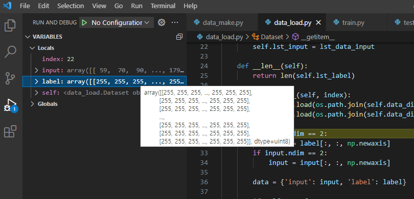
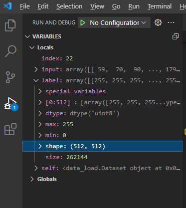
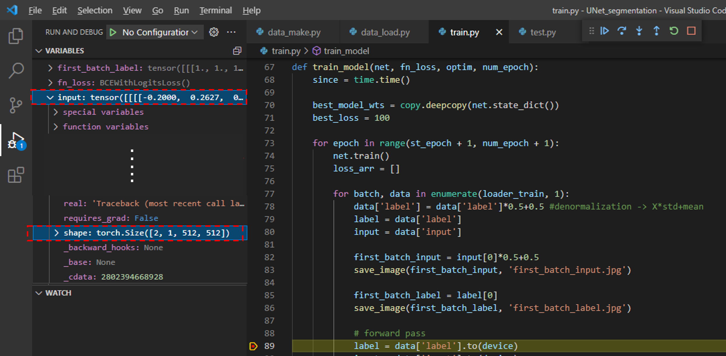
먼저, 아래 부분(89번 line)에 breakpoint를 걸어주어 input 데이터의 shape을 살펴보면, (batch, Channel, Height, Width)와 같은 형태로 구성되어 있는걸 확인하실 수 있습니다. 

그럼 input, label의 각각 첫 번째 batch 이미지를 따로 저장시킬 코드를 추가하겠습니다.

우선 input 데이터에서도 normalize가 적용된 상태이기 때문에 denormalize를 해줍니다. (←"input[0]*0.5+0.5")

그리고 첫 번째 batch 이미지에 해당하는 데이터 값은 "input[0]*0.5+0.5", "label[0]"인데, 현재 데이터 형식은 torch tensor입니다.

torch tensor 형식에서 곧 바로 이미지를 저장하기 위해서는 "torchvision.utils"에서 제공하는 save_image()를 이용하면 됩니다.

      for batch, data in enumerate(loader_train, 1):
            data['label'] = data['label']*0.5+0.5 #denormalization -> X*std+mean
            label = data['label']
            input = data['input']
			
            #################코드가 추가된 부분###################
            first_batch_input = input[0]*0.5+0.5
            save_image(first_batch_input, 'first_batch_input.jpg')

            first_batch_label = label[0]
            save_image(first_batch_label, 'first_batch_label.jpg')
            #######################################################

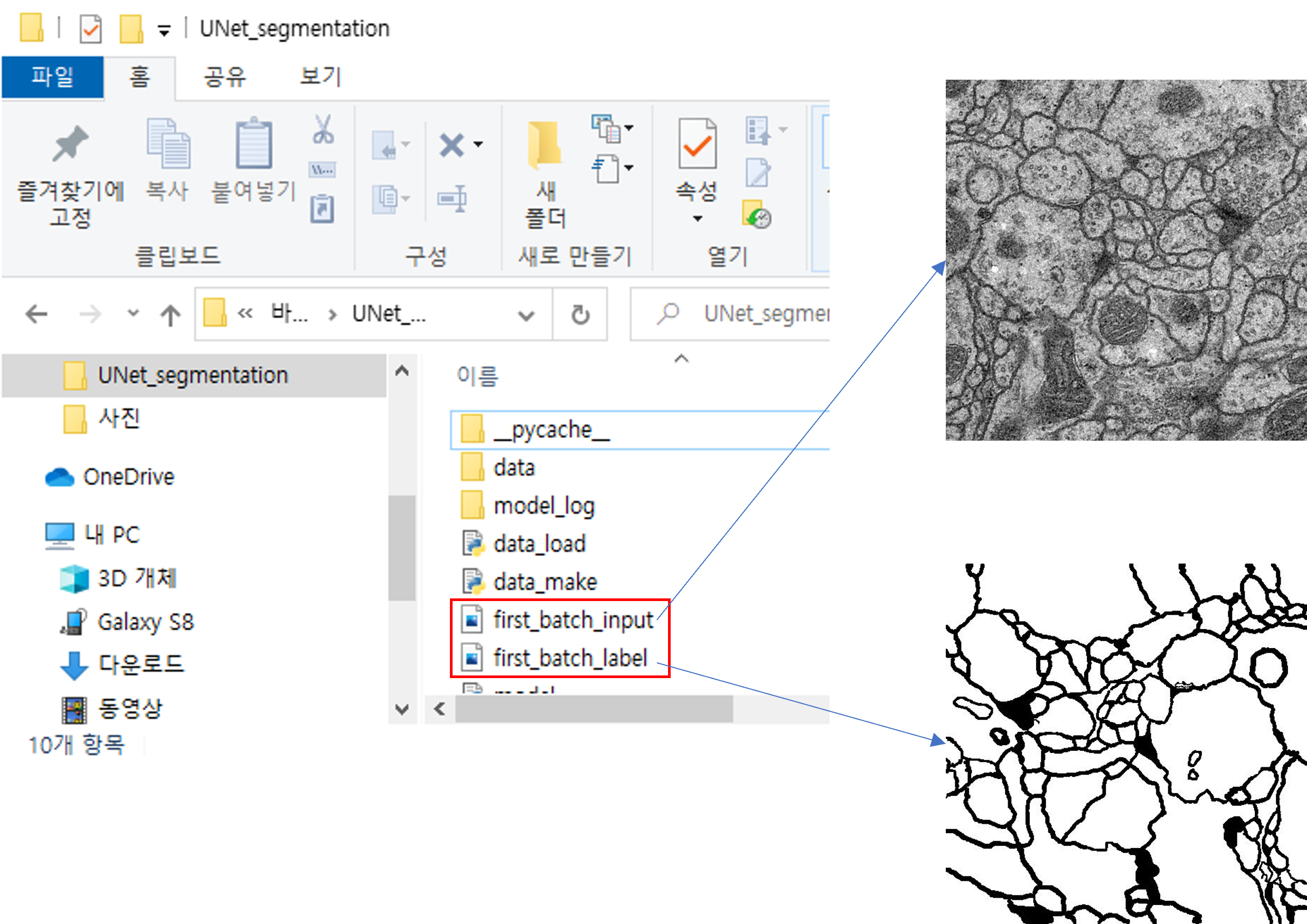
코드를 실행하고 저장된 이미지를 살펴보겠습니다.

input 데이터의 이미지와 label 데이터의 이미지가 일치하지 않는게 보이시나요? 어느 한쪽이 flip이 안 됐다는 정도는 파악할 수 있을겁니다.

이렇게 나오는 이유를 찾기 위해 transforms.RandomHorizontalFlip 코드를 살펴보았습니다.

(↓↓↓transforms.RandomHorizontalFlip API ↓↓↓)

https://pytorch.org/vision/stable/_modules/torchvision/transforms/transforms.html#RandomHorizontalFlip

해당 API를 차례대로 살펴보겠습니다.

앞서 input, label에 서로다른 augmenation이 적용된 이유는 torch.rand() 때문입니다. 왜 torch.rand() 때문이었는지 좀 더 자세히 설명해보도록 하겠습니다.

 torch.rand()이라는 함수에 대한 설명은 아래와 같습니다.

• Returns a tensor filled with random numbers from a uniform distribution on the interval [0, 1)[0,1)

(↓↓↓torch.rand↓↓↓)

https://pytorch.org/docs/stable/generated/torch.rand.html

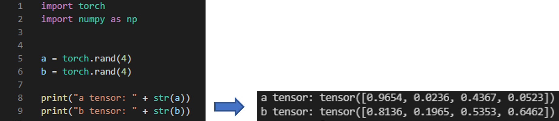
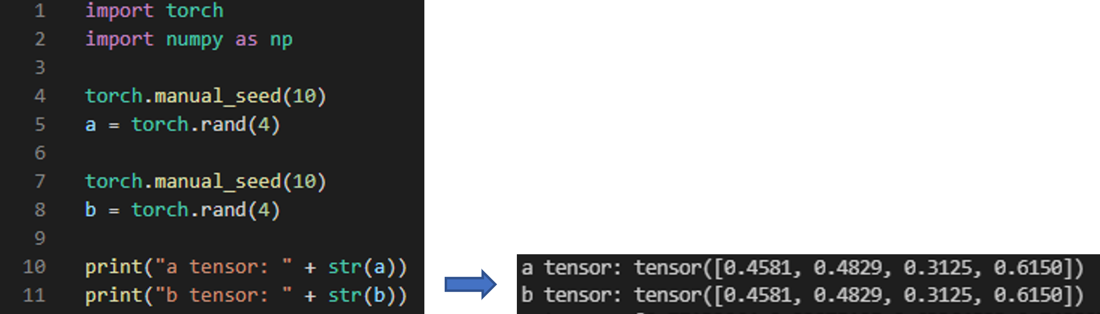
torch.rand(1)은 데이터가 1차원 형태이며 0~1 사이의 값 중 하나를 출력한다는 뜻입니다. 

만약, 4차원 형태를 나타내려면 아래와 같이 코딩해주면 됩니다.

위의 코드를 결과를 살펴보면 torch.rand를 실행시켜 줄 때 마다 난수가 발생하기 때문에 a, b에 들어가는 값들이 전부다른걸 보실 수 있습니다.

위와 같은 사실을 기반으로 "data_load.py"에 구현되어 있는 아래 코드를 살펴보겠습니다.

우선 data['input']에 해당하는 데이터에 transform이 진행되는 과정을 살펴보겠습니다. → self.transform(data['input'])

        if self.transform:  
            #torch.manual_seed(10)
            data['input'] = self.transform(data['input'])

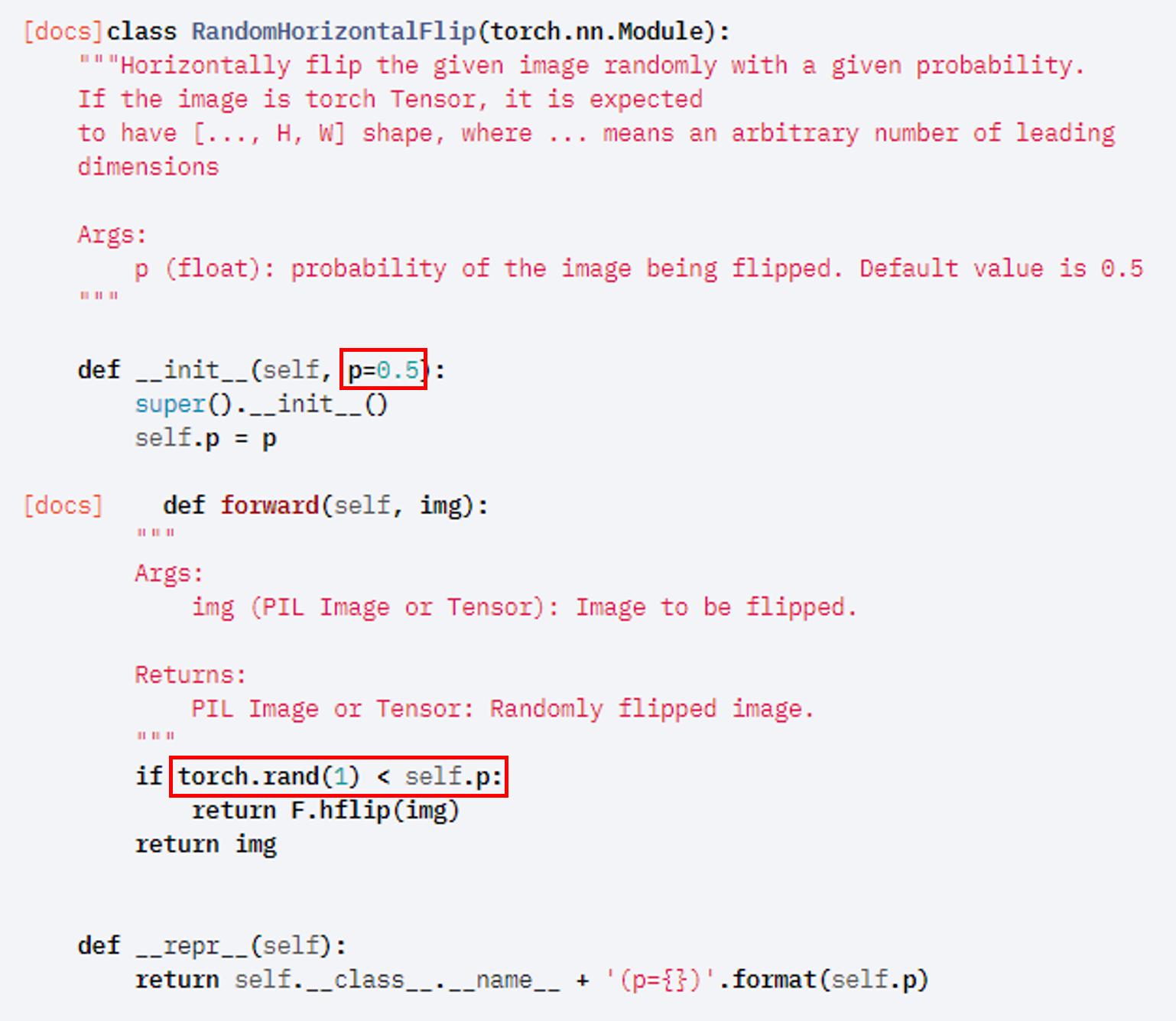
앞서 transforms.Compose에 구현된 것 중하나가 RandomHorizontalFlip()인데, 이 부분이 아래와 같은 코드를 기반으로 수행이 될 겁니다. 그런데 보면, torch.rand(1)를 통해 난수가 발생하는 걸 볼 수 있죠? 만약 여기서 0.3이라는 값이 생성되면 "p=0.5" 기준에 의해 RandomHorizontalFlip() 방식의 augmentation이 진행되지 않을 것입니다.

이때 label 데이터에서도 RandomHorzontalFlip()이 적용이 되는데 (by "self.transform(data['label'])"),  torch.rand(1)에서 생성된 값(=난수)가 0.6이면, label에는 RandomHorzontalFlip()이 적용되게 됩니다.

        if self.transform:  
            #torch.manual_seed(10)
            data['input'] = self.transform(data['input'])
            
        if self.transform:
            #torch.manual_seed(10)
            data['label'] = self.transform(data['label'])

그래서 "그림7"과 같은 결과를 보이게 됩니다.

이러한 문제를 해결하기 위해서는 "torch.rand(1)"를 통해 생성되는 난수를 고정시켜주어야 합니다.

난수를 고정시키는 방법은 간단합니다. 아래와 "그림10"처럼 난수가 생성되기 전에  seed 값을 고정시켜주면 됩니다. 그러면, torch.rand()를 통해 생겨나는 난수 값들이 고정됩니다.

위와 같은 방식을 통해 self.transform(data['input']), self.trasnform(data['label'])에서 augmentation 시, 발생되는 난수 값이 (by "torch.rand()") 동일해집니다.  즉, input, label 모두 동일한(일치한) augmentation을 제공해주게 됩니다.

        if self.transform:  
            torch.manual_seed(10)
            data['input'] = self.transform(data['input'])
            
        if self.transform:
            torch.manual_seed(10)
            data['label'] = self.transform(data['label'])

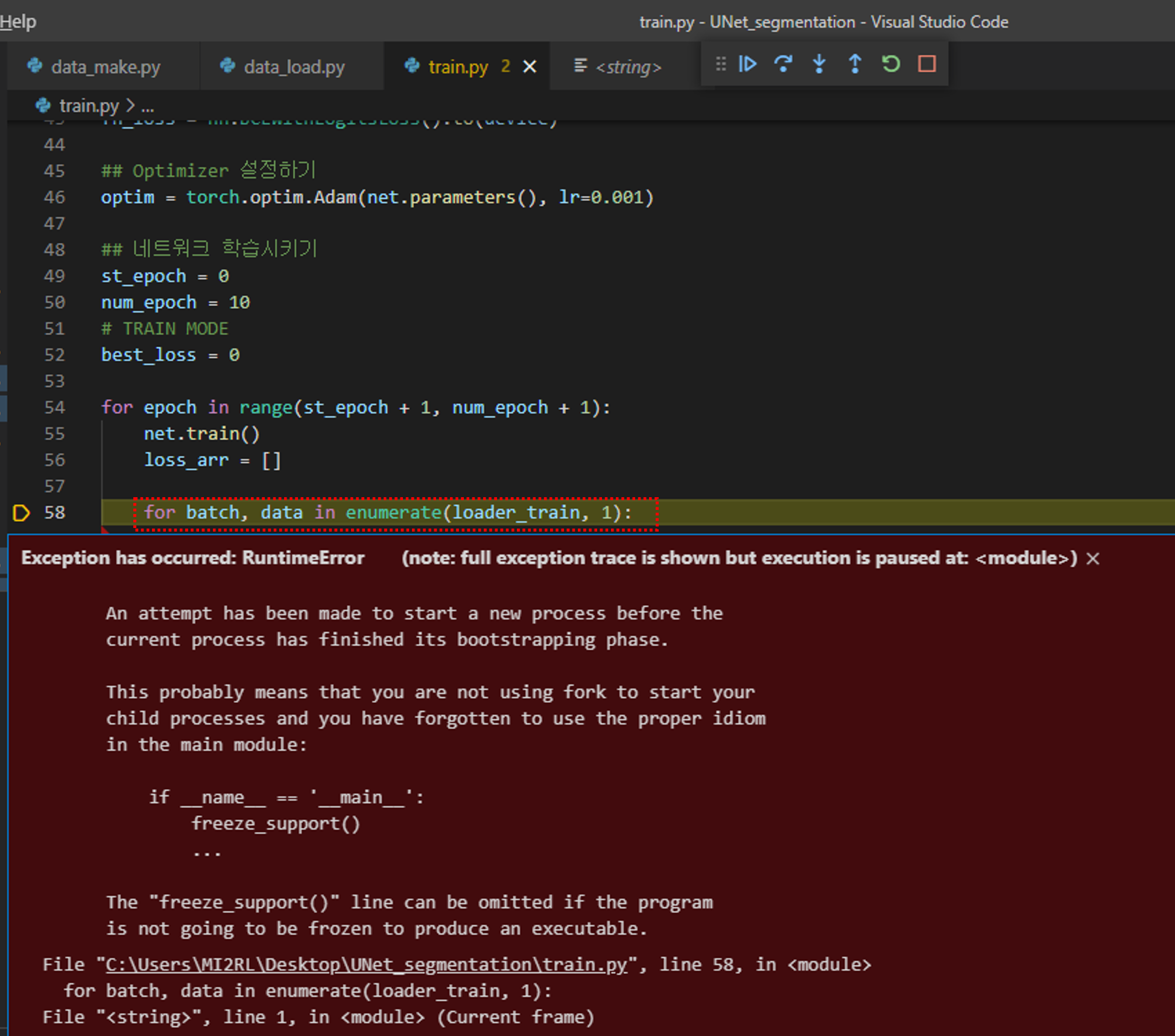
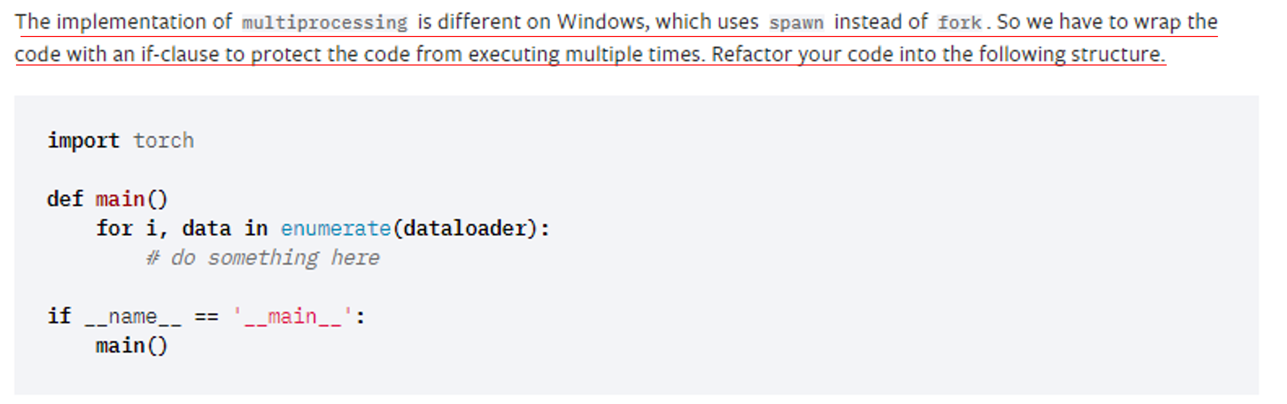
3. freeze_support() 에러

데이터 로드와 관련된 모든 준비가 완료되었습니다.

그럼 "train.py" 코드를 실행해보죠.

만약 앞서 제가 설명드린 코드가 아닌 유튜브 강의에서 설명한 코드로 실행했을 때 리눅스에서 실행하셨다면 큰 문제없이 실행됐겠지만, 만약 윈도우에서 실행시키셨다면 아래와 같은 에러 메시지를 만나실 수 있습니다.

아래 코드를 한 번 살펴보겠습니다. 

DataLoader에 num_workers가 보이시나요?

from torchvision import transforms

transform_train = transforms.Compose([
    transforms.ToPILImage(), 
    transforms.RandomHorizontalFlip(),
    transforms.RandomVerticalFlip(), 
    transforms.ToTensor(),
    transforms.Normalize(mean=0.5, std=0.5)])
    
dataset_train = Dataset(data_dir=os.path.join(data_dir, 'train'), transform=transform_train)
loader_train = DataLoader(dataset_train, batch_size=batch_size, shuffle=True, num_workers=0)

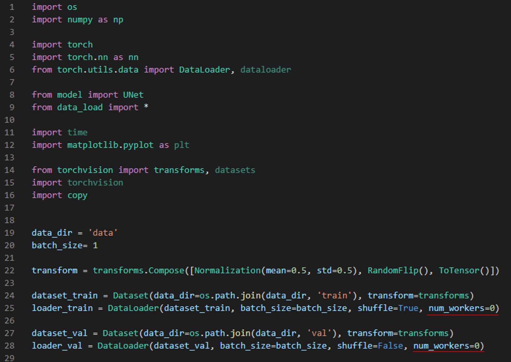
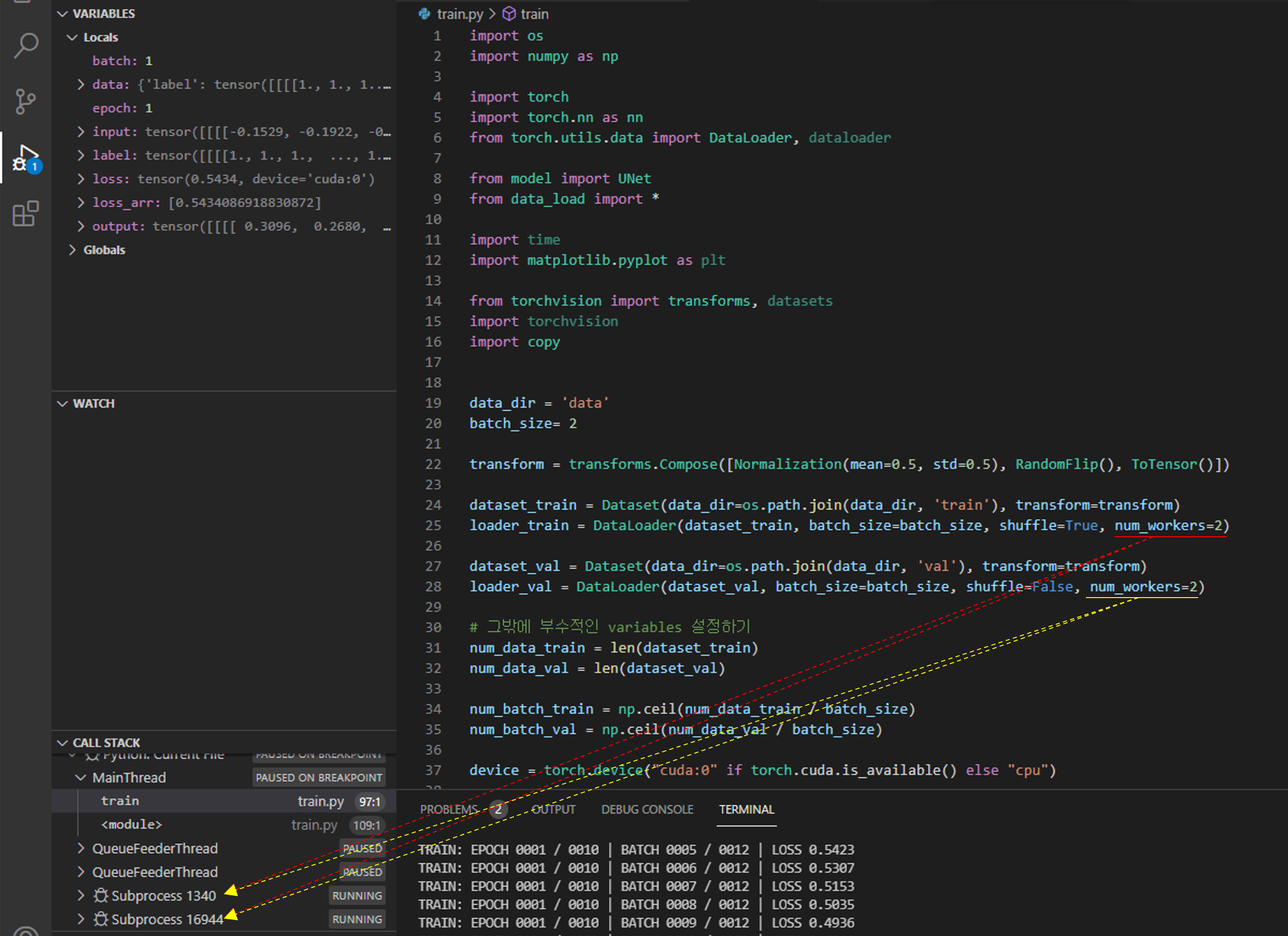
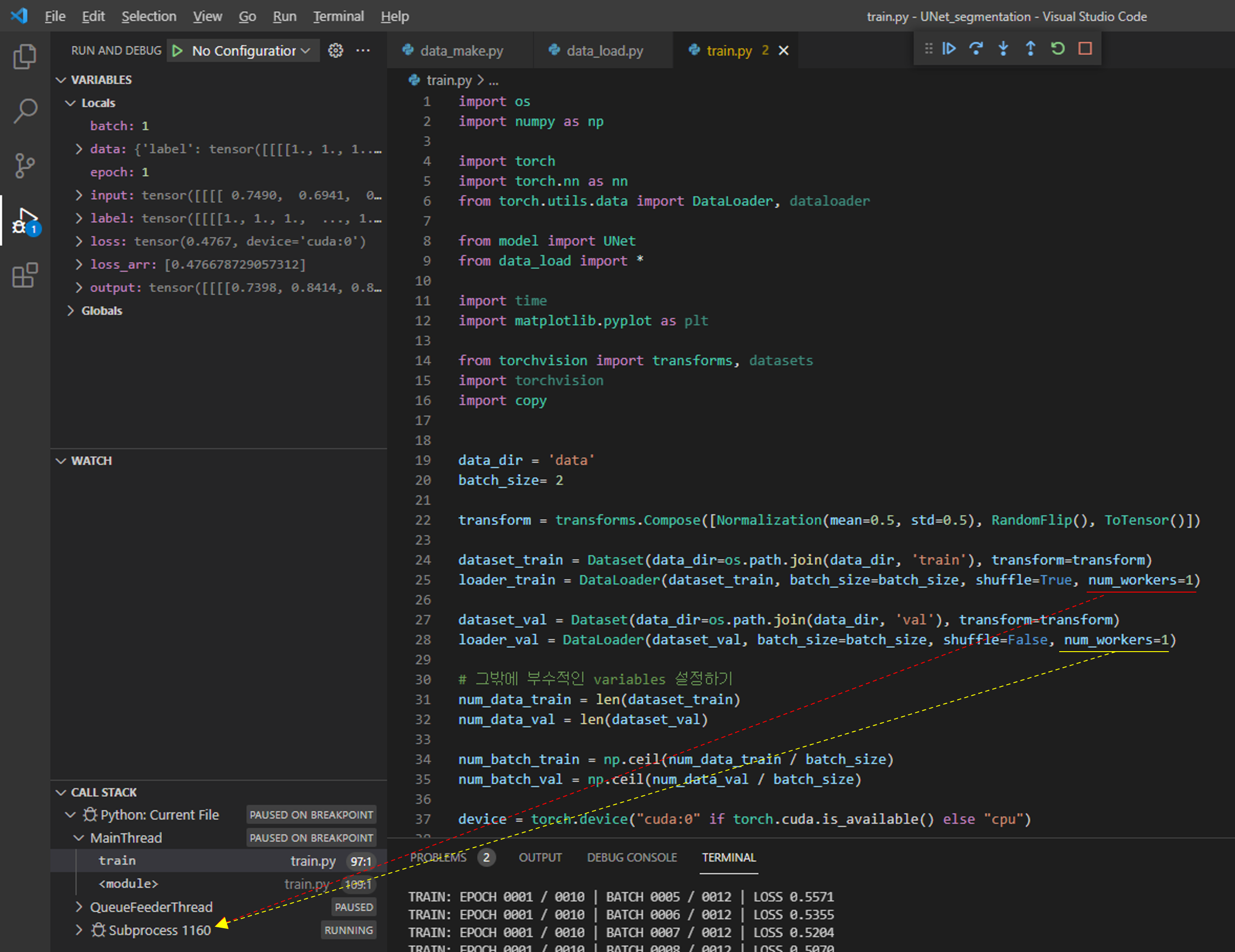
num_workers는 GPU에 학습 이미지를 업로드하기 위해서 사용되는 CPU의 process 개수입니다. 

쉽게 말해 GPU 학습 이미지를 업로드 하기 위해서는 결국 CPU가 중간 다리 역할을 해줘야 하는데, 이때 num_workers를 크게 설정해주면 GPU에 학습 이미지를 업로드하는데 관여하는 process도 많아지겠죠. 이렇게 되면 결국 학습 이미지 업로드 속도도 빨라질겁니다.

(↓↓↓num_workers에 대해서 설명한 글↓↓↓)

https://89douner.tistory.com/287?category=994842 

앞서 "그림11"에서 설명한 에러가 발생하는 이유는 아래의 사이트에서 설명하고 있습니다.

https://pytorch.org/docs/stable/notes/windows.html#usage-multiprocessing

요약해 설명하자면 "Dataload"를 수행시키기 위해서는 multi-process (by "num_workers")를 이용하는데, 이것이 리눅스가 아닌 window에서 사용하기 위해서는 아래와 같이 특정 작업을 해주어야 한다고 합니다.

3-1) 첫 번째 에러 수정 방법

첫 번째 방식은 매우 간단합니다.

그냥 num_workers 부분을 0으로 세팅해주면 됩니다.

3-1) 두 번째 에러 수정 방법

두 번째 에러 수정 방법은 "그림11"에서 제안한대로 코드를 변경시켜 주면 됩니다.

아래 그림14처럼 "train.py"에서 "def train()"함수 부분을 만들어주고 (←유튜브 강의에서는 train()함수를 따로 정의하진 않고 있습니다) training에 해당되는 코드를 옮겨줍니다. 그리고, 마지막 코드에 추가로 main관련 코드를 작성해줍니다. 

import os
import numpy as np

import torch
import torch.nn as nn
from torch.utils.data import DataLoader

from model import UNet
from data_load import *

import time

from torchvision import transforms
import albumentations as A

import copy
from torchvision.utils import save_image

data_dir = 'data'
batch_size= 2


transform_train = transforms.Compose([
    transforms.ToPILImage(), 
    transforms.RandomHorizontalFlip(),
    transforms.RandomVerticalFlip(), 
    transforms.ToTensor(),
    transforms.Normalize(mean=0.5, std=0.5)])


transform_val = transforms.Compose([
    transforms.ToPILImage(), 
    transforms.RandomHorizontalFlip(), 
    transforms.ToTensor(),
    transforms.Normalize(mean=0.5, std=0.5)
    ])


dataset_train = Dataset(data_dir=os.path.join(data_dir, 'train'), transform=transform_train)
loader_train = DataLoader(dataset_train, batch_size=batch_size, shuffle=True, num_workers=2)

dataset_val = Dataset(data_dir=os.path.join(data_dir, 'val'), transform=transform_val)
loader_val = DataLoader(dataset_val, batch_size=batch_size, shuffle=False, num_workers=2)


# 그밖에 부수적인 variables 설정하기
num_data_train = len(dataset_train)
num_data_val = len(dataset_val)

num_batch_train = np.ceil(num_data_train / batch_size)
num_batch_val = np.ceil(num_data_val / batch_size)

device = torch.device("cuda:0" if torch.cuda.is_available() else "cpu")

## 네트워크 생성하기
net = UNet().to(device)

## 손실함수 정의하기
fn_loss = nn.BCEWithLogitsLoss().to(device)

## Optimizer 설정하기
optim = torch.optim.Adam(net.parameters(), lr=1e-3)

## 네트워크 학습시키기
st_epoch = 0
num_epoch = 30
# TRAIN MODE

def train_model(net, fn_loss, optim, num_epoch):
    since = time.time()

    best_model_wts = copy.deepcopy(net.state_dict())
    best_loss = 100

    for epoch in range(st_epoch + 1, num_epoch + 1):
        net.train()
        loss_arr = []

        for batch, data in enumerate(loader_train, 1):
            data['label'] = data['label']*0.5+0.5 #denormalization -> X*std+mean
            label = data['label']
            input = data['input']

            # first_batch_input = input[0]*0.5+0.5
            # save_image(first_batch_input, 'first_batch_input.jpg')

            # first_batch_label = label[0]
            # save_image(first_batch_label, 'first_batch_label.jpg')

            # forward pass
            label = data['label'].to(device)
            input = data['input'].to(device)

            output = net(input)

            # backward pass
            optim.zero_grad()

            loss = fn_loss(output, label)
            loss.backward()

            optim.step()

            # 손실함수 계산
            loss_arr += [loss.item()]

            print("TRAIN: EPOCH %04d / %04d | BATCH %04d / %04d | LOSS %.4f" %
                (epoch, num_epoch, batch, num_batch_train, np.mean(loss_arr)))


        with torch.no_grad():
            net.eval()
            loss_arr = []

            for batch, data in enumerate(loader_val, 1):
                data['label'] = data['label']*0.5+0.5 #denormalization -> X*std+mean

                # forward pass
                label = data['label'].to(device)
                input = data['input'].to(device)

                output = net(input)

                # 손실함수 계산하기
                loss = fn_loss(output, label)

                loss_arr += [loss.item()]

                print("VALID: EPOCH %04d / %04d | BATCH %04d / %04d | LOSS %.4f" %
                        (epoch, num_epoch, batch, num_batch_val, np.mean(loss_arr))) 

            epoch_loss = np.mean(loss_arr)

            # deep copy the model
            if epoch_loss < best_loss:
                best_loss = epoch_loss
                best_model_wts = copy.deepcopy(net.state_dict())

        print()
    
    time_elapsed = time.time() - since
    print('Training complete in {:.0f}m {:.0f}s'.format(
        time_elapsed // 60, time_elapsed % 60))
    print('Best val loss: {:4f}'.format(best_loss))

    # load best model weights
    net.load_state_dict(best_model_wts)
    return net

if __name__ == '__main__':
    model_ft = train_model(net, fn_loss, optim, num_epoch)
    torch.save(model_ft.state_dict(), './model_log/model_weights.pth')

위와 같이 변경해주고 실행시켜주면 num_workers에 따라 subprocess가 발생하는걸 확인하실 수 있습니다.

지금까지 pytorch에서 제공해주는 transform을 이용하기 위해 변경시켜야 할 부분들을 설명했습니다.

감사합니다.

안녕하세요.

이번 글에서는 Segmentation을 하기 위해 데이터셋을 어떻게 세팅해놓는지에 대해 설명하려고 합니다.

코드는 아래 사이트를 기반으로 수정하였으니 아래 영상을 먼저 참고하시면 글을 이해하시는데 도움이 될 것으로 생각됩니다.

https://www.youtube.com/watch?v=fWmRYmjF-Xw 

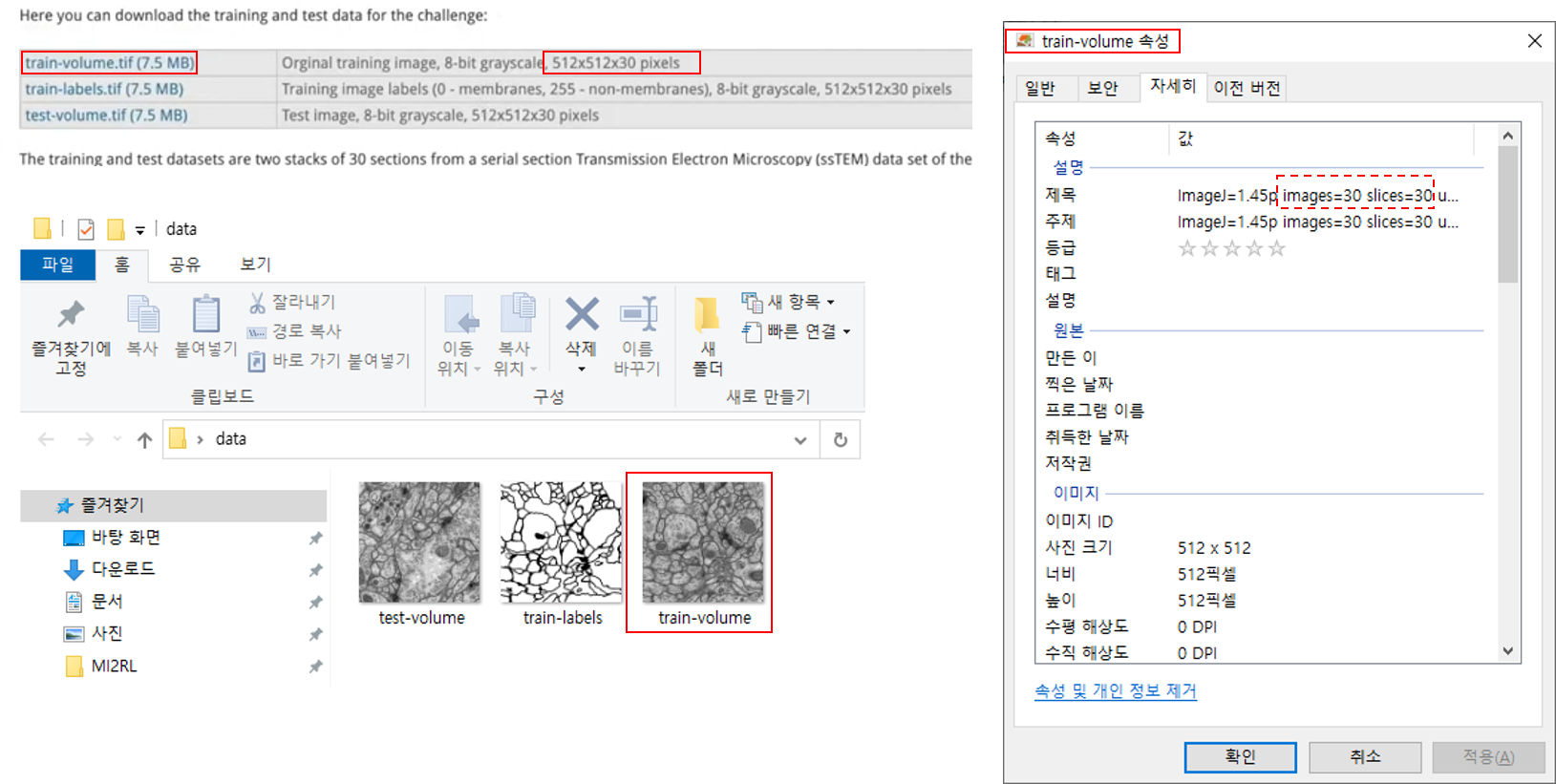
1. 데이터 다운받기 (Feat. ISBI 2012 EM segmentation Challenge)

보통 segmentation을 하기 위한 public 데이터들은 Kaggle, MICCAI 같은 곳에서 열리는 segmentation challenge에서 구할 수 있습니다. 또는 과거에 진행되었거나 현재에 진행되는 다른 segmentation challenge에서도 구할 수 있습니다.

보통 유명한 데이터셋들 중에 크기가 작은 데이터들은 github에 올려놓는 경우도 있습니다.

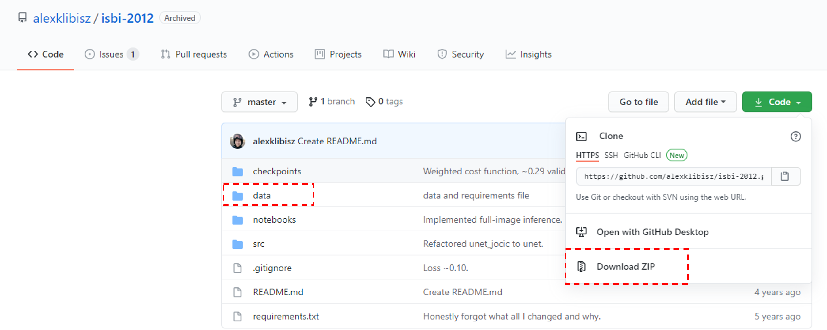
이번 글에서는 "ISBI 2012 EM segmentation Challenge"에서 사용되었던 membrane 데이터셋을 github에서 다운받아 사용해보려고 합니다.

방법은 간단합니다.

먼저 "ISBI 2012 github", "ISBI 2012 segmentation" 등의 키워드를 구글에 검색하시면 다양한 github 사이트가 노출이 될 겁니다.

제가 찾은 사이트는 아래 사이트인데, 먼저 아래 사이트에 접속해보도록 하겠습니다.

https://github.com/alexklibisz/isbi-2012

해당 사이트에 접속하시면 data 폴더에 "ISBI 2012 EM" 데이터들이 들어 있다는걸 확인할 수 있습니다.

아래 "그림1"처럼 github repository를 다운 받습니다 ("우측 상단에 Code를 누른 후, Download ZIP을 클릭해 주세요") 

다운받은 데이터는 아래 그림과 같이 되어 있습니다.

해당 데이터에 데한 정보는 다음과 같습니다.

• train-volume.tif : input image data for training
• train-label.tif : label image data for training
• test-volume.tif : test image data

위의 세 가지 데이터 모두 512×512×30으로 설정되어 있습니다.

여기서 "30"이 의미하는 것은 무엇일까요?

해당 이미지 속성을 보면 slices=30이라는 부분이 눈에 띕니다. 

즉, "train-volume.tif" 이미지 파일은 30개의 별도의 이미지를 포함하고 있다는 뜻인데, 이것을 그림으로 표현하면 아래와 같습니다.

2. 개별 이미지 추출하기

앞서 다운받은 이미지 형식이 무엇을 의미하는지 설명했습니다.

그럼 이제부터 "512×512×30" 형식의 이미지에서 개별 이미지들을 따로 추출해보겠습니다.

먼저, UNet_segmentation이라는 폴더를 만든 후, 이전에 다운 받은 data 폴더를 복사, 붙여놓기 합니다.

그리고, 개별 이미지들을 저장시킬 디렉터리 ('test', 'train', 'val') 폴더를 만들어 줍니다.

추가적으로 각각의 폴더 ('train', 'val', 'test') 에 input, label 데이터를 저장시킬 별도의 폴더를 아래와 같이 만들어 줍니다.

Visual Studio에서 위의 개별 이미지들을 나누는 코드를 작성해보도록 하겠습니다.

우선 전체 코드를 보여드리면 아래와 같습니다.

## 필요한 패키지 등록
import os
import numpy as np
from PIL import Image
import matplotlib.pyplot as plt

## 1) 데이터 불러오기
dir_data = './data'

name_label = 'train-labels.tif'
name_input = 'train-volume.tif'

img_label = Image.open(os.path.join(dir_data, name_label))
img_input = Image.open(os.path.join(dir_data, name_input))

ny, nx = img_label.size
nframe = img_label.n_frames

## 2) training, validation, test 이미지 데이터 개수 정해주기
nframe_train = 24
nframe_val = 3
nframe_test = 3

dir_save_train_input = os.path.join(dir_data, 'train/input')
dir_save_train_label = os.path.join(dir_data, 'train/label')
dir_save_val_input = os.path.join(dir_data, 'val/input')
dir_save_val_label = os.path.join(dir_data, 'val/label')

dir_save_test_input = os.path.join(dir_data, 'test/input')
dir_save_test_label = os.path.join(dir_data, 'test/label')

## 3) 512x512x30에서 선별할 frame shuffle해서 추출하기 
id_frame = np.arange(nframe)
np.random.shuffle(id_frame) #사실 shuffle은 굳이 안해줘도 됨

## 4) 24개의 training data (input, label)를 추출하기
offset_nframe = 0

for i in range(nframe_train):
    img_label.seek(id_frame[i + offset_nframe])
    img_input.seek(id_frame[i + offset_nframe])

    # img_label.save(os.path.join(dir_save_train, 'label_%03d.tif' % i))
    # img_input.save(os.path.join(dir_save_train, 'input_%03d.tif' % i))

    label_ = np.asarray(img_label)
    input_ = np.asarray(img_input)

    np.save(os.path.join(dir_save_train_label, 'label_%03d.npy' % i), label_)
    np.save(os.path.join(dir_save_train_input, 'input_%03d.npy' % i), input_)

## 5) 3개의 validation data (input, label)를 추출하기
offset_nframe = nframe_train

for i in range(nframe_val):
    img_label.seek(id_frame[i + offset_nframe])
    img_input.seek(id_frame[i + offset_nframe])

    # img_label.save(os.path.join(dir_save_val, 'label_%03d.tif' % i))
    # img_input.save(os.path.join(dir_save_val, 'input_%03d.tif' % i))

    label_ = np.asarray(img_label)
    input_ = np.asarray(img_input)

    np.save(os.path.join(dir_save_val_label, 'label_%03d.npy' % i), label_)
    np.save(os.path.join(dir_save_val_input, 'input_%03d.npy' % i), input_)

## 6) 3개의 test data (input, label)를 추출하기
offset_nframe = nframe_train + nframe_val

for i in range(nframe_test):
    img_label.seek(id_frame[i + offset_nframe])
    img_input.seek(id_frame[i + offset_nframe])

    # img_label.save(os.path.join(dir_save_test, 'label_%03d.tif' % i))
    # img_input.save(os.path.join(dir_save_test, 'input_%03d.tif' % i))

    label_ = np.asarray(img_label)
    input_ = np.asarray(img_input)

    np.save(os.path.join(dir_save_test_label, 'label_%03d.npy' % i), label_)
    np.save(os.path.join(dir_save_test_input, 'input_%03d.npy' % i), input_)

2-1) Image 모듈

사실 위에 있는 코드를 따로 설명한다기보다 Image 모듈의 attribute, function 들을 소개하는 것이 더 좋을 것 같아 아래 링크를 첨부하도록 하겠습니다.

https://89douner.tistory.com/310

https://89douner.tistory.com/309?category=1002521 

2-2) training dataset

위의 코드에서 한 가지 부분만 말씀드리면 "train-volume.tif" 데이터에는 30개의 별도 이미지가 있는데, 이중에서 24개는 training dataset, 3개는 validatin dataset, 3개는 test dataset으로 이용한다는 점입니다.

2-3) numpy 형태로 저장하는 이유

위의 코드에서 개별 이미지를 numpy 형태로 저장하는 것을 볼 수 있습니다.

numpy 형태로 저장하는 이유는 현재 이미지 shape이 (512, 512) 이기 때문입니다.

    label_ = np.asarray(img_label)
    input_ = np.asarray(img_input)

    np.save(os.path.join(dir_save_train, 'label_%03d.npy' % i), label_)
    np.save(os.path.join(dir_save_train, 'input_%03d.npy' % i), input_)

(아래와 같이 "a=label_shape" 코드를 추가한 후,  살펴 보면 (512,512) 형태임을 알 수 있습니다) 

위의 이미지 형태에서 빠진 것 중 하나가 channel 정보입니다.

Pytorch의 딥러닝 모델을 학습시키기 위해서는 입력 데이터의 가로, 세로 길이와 channel (1=gray, 3=rgb) 정보가 들어있어야 합니다.

하지만 위의 shape을 통해 확인한 결과 현재는 "(H,W)=(이미지 높이, 이미지 너비)" 구조입니다.

그래서 이러한 구조를  "(H,W,C) = (이미지 높이, 이미지 너비, 이미지 채널)" 로 만들어 주어야 합니다.

numpy 형식을 이용하면 현재 "(H,W)"형태의 구조에서 축 하나를 쉽게 늘려 "(H,W,C)" 형태로 만들 수 있게 됩니다.

위의 코드 중에 아래와 같이 주석처리된 부분이 있는데, 만약 본인이 numpy가 아닌 이미지 형식으로 저장시켜 보고 싶다면 아래 주석 부분을 제거해주시면 됩니다. (그럼 개별 이미지들이 tif 형식으로 저장되 직접 확인하실 수 있습니다)

    # img_label.save(os.path.join(dir_save_train, 'label_%03d.tif' % i))
    # img_input.save(os.path.join(dir_save_train, 'input_%03d.tif' % i))

※사실 R,G,B 이미지였다면 (512,512,3) 형태로 저장이 되었을 것이기 때문에, 따로 numpy로 저장할 필요가 없습니다. 하지만, 현재 다루고 있는 이미지가 Gray scale을 따른다면 numpy 형태로 저장할 필요가 있습니다. (사실, gray scale 이미지도 엄격하게 표현하려면 (512,512,1)로 표현되어야 하지만, 이미지에서는 channel에 해당하는 1 부분을 생략하고 (512,512)로 표현하는 경우가 있습니다.)

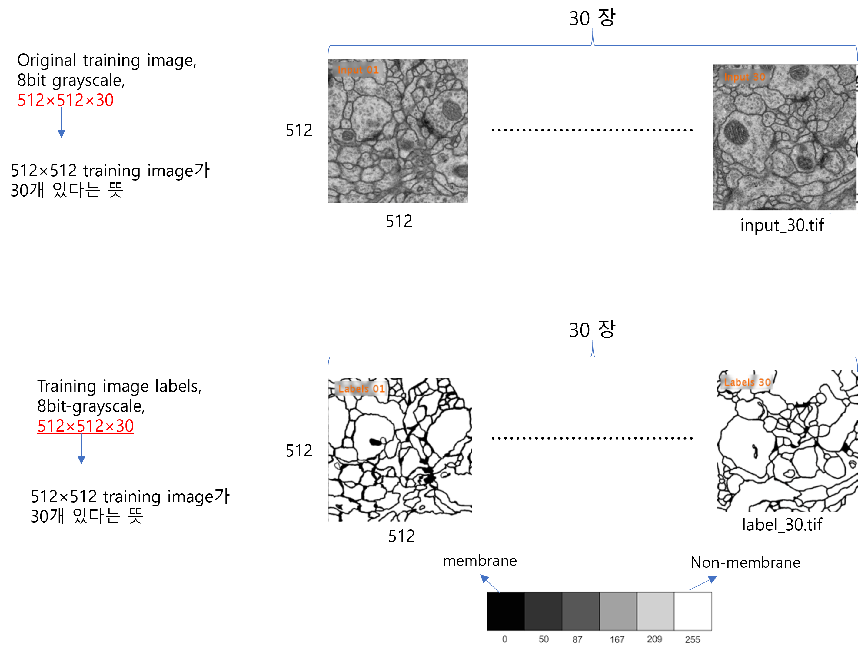
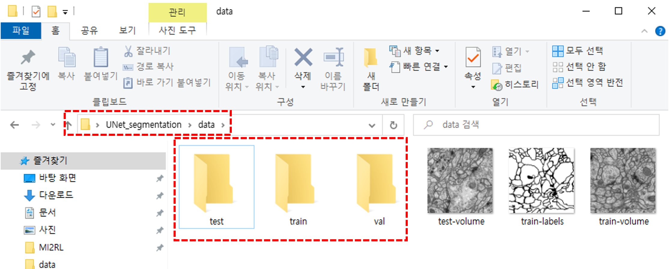
※이 글에서는 slice형태로 이미지가 묶여서 나오기 때문에 지금과 같이 별개의 이미지로 분리하는 작업을 거쳤지만, 만약 이미지 데이터들이 3차원의 별도의 이미지로 제공이 될 경우는 지금까지 설명했던 코드를 구현할 필요는 없습니다.

※하지만, 의료 영상에서 다루는 CXR, CT, MRI 이미지들은 대부분 Gray scale이 많기 때문에 medical 분야에서 인공지능을 하시는 분들은 위의 코드를 잘 숙지하고 있으시면 많은 도움이 될 거라 생각합니다.

감사합니다. 

안녕하세요.

이번 Pytorch 기반의 segmentation 코드 설명은 UNet을 기반으로 하려합니다.

아래 강의를 참고로 설명을 하니 먼저 아래 강의를 들으셔도 좋을 것 같습니다.

https://www.youtube.com/watch?v=fWmRYmjF-Xw 

https://github.com/hanyoseob/youtube-cnn-002-pytorch-unet

안녕하세요.

이번 글에서는 Pillow 패키지의 가장 기본이 되는 모듈인 Image 모듈에 대해서 설명하려고 합니다.

1. Image 모듈이란?

Image 모듈은 기본적으로 이미지 파일을 로드하거나 새로운 이미지를 생성하는 기능들을 제공해줍니다.

"The module also provides many factory functions, including loading images from files and creating new images."

모듈이라는 것은 크게 두 가지 요소로 구성되어 있다고 볼 수 있습니다.

1. attribute = 속성
2. function = 함수

먼저 Image 모듈 reference 사이트에 접속해서 어떤 attribute이 있는지 살펴보겠습니다.

(↓↓↓Image Module reference site↓↓↓)

https://pillow.readthedocs.io/en/stable/reference/Image.html

2. Image 모듈 함수(=function) (Feat. attribute)

2-1. Image.open()

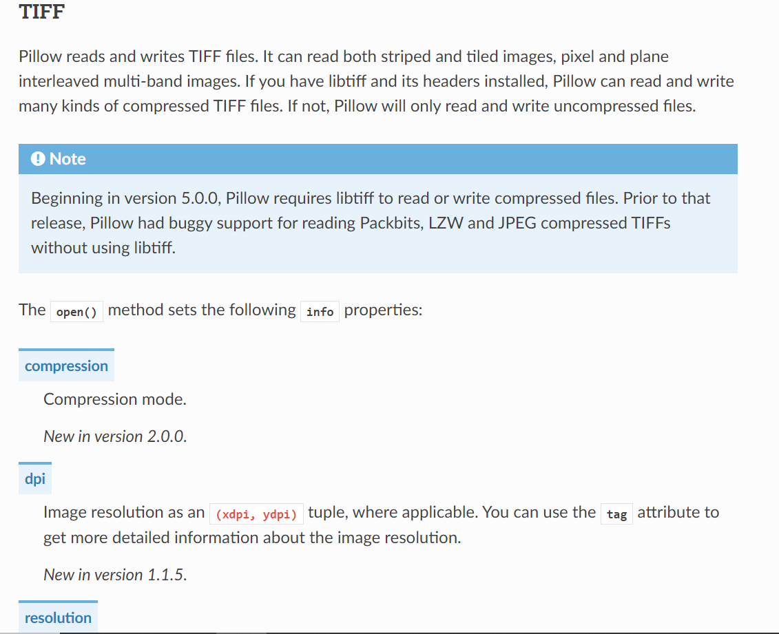
Image 모듈 reference site를 들어가 보면 첫 번째로 보이는 함수가 open()입니다.

아래 설명을 통해 보자면 open()이라는 함수는 어떤 이미지 파일을 단지 identification(확인) 하는 역할을 수행합니다. 

즉, 이미지 데이터를 읽어드린 것이 아니라 단지 이미지 파일에 대한 몇 가지 (메타)정보를 확인합니다.

예를 들어, 아래와 같이 Image.open() 함수를 통해 리턴 받은 img_input 값들을 살펴보면 Image 모듈의 기본적인 attribute 값들 (=filename, size, width, height, format) 과 그 외에 현재 이미지와 관련한 다양한 정보들을 포함하고 있다는걸 확인할 수 있습니다.

(↓↓↓ Image 모듈의 다양한 attribute들 ↓↓↓)

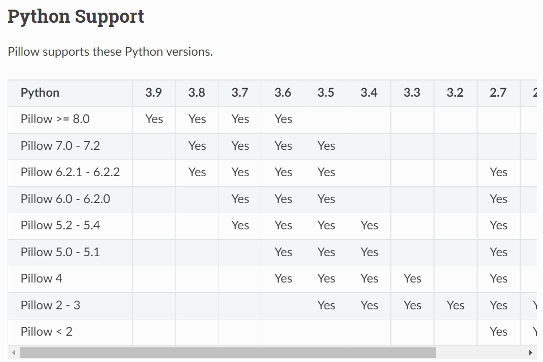
image 모듈은 굉장히 다양한 image file format을 지원합니다. 아래 링크에 접속하면 지원가능한 format 형식들이 나옵니다.

"The open() function identifies files from their contents. When an image is opened from a file, only that instance of the image is considered to have the format."

https://pillow.readthedocs.io/en/stable/handbook/image-file-formats.html#tiff

위에서 사용한 이미지 파일의 format은 tiff인데, 위 링크에 들어가면 아래 화면 처럼 TIFF 파일 형식을 찾아볼 수 있습니다.

만약 TIFF 파일을 image.open()으로 읽어들이면 tiff 이미지와 관련된 다양한 값들을 리턴받을 수 있는데, 이러한 값들에 대한 설명이 아래와 같이 나옵니다.

(↓↓↓ TIFF file format (Feat. open()) ↓↓↓)

https://pillow.readthedocs.io/en/stable/handbook/image-file-formats.html#tiff

image.open() 함수의 설명 중에는 또 이러한 아래와 같은 표현이 있습니다.

"The file object must be opened in binary mode." 

여기서 말하는 binary model란 "binary representation of the pixels"라고 보시면 됩니다.

이진 파일이란 컴퓨터는 읽을 수 있으나 사람을 읽지 못하는 파일입니다. 

보통 binary mode로 읽으면 byte 단위로 읽게되는 데, 아래 "data" 값을 보면 확인 할 수 있습니다. 

위와 같은 binary 관련 내용은 아래를 참고해주세요!

https://ballentain.tistory.com/50

https://stackoverflow.com/questions/48367128/string-to-bytes-python-without-change-in-encoding

https://stackovergo.com/ko/q/980400/convert-binary-files-into-ascii-in-python

Image.open() 함수의 리턴 값은 Image 객체입니다.

즉, 리턴 받은 값에서 다시 Image 모듈의 function, attribute를 사용할 수 있다는 뜻입니다.

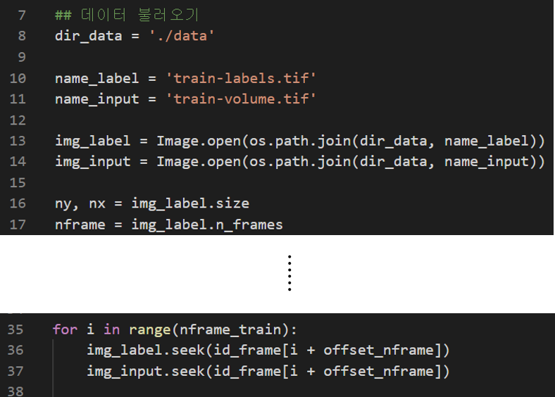
예를 들어, 아래 코드와 같이 Image.open()를 통해 Image 객체를 리턴 받은 img_input가 Image 모듈의 함수 중 하나인 seek() 을 이용할 수 있다는걸 확인 할 수 있습니다.

Image.open() 함수의 parameter 부분에 "fp" 설명을 보면 마지막 부분에 "the file object must implement "read()", "seek()", "tell()"같은 함수를 사용해야 실제로 이미지 데이터를 load할 수 있다고 합니다. (이 부분은 뒤에서 "file.seek" 함수 를 설명할 때 더 자세히 하도록 하겠습니다)

2-2. Image.seek()

앞서 실제 이미지 데이터를 load 하는 함수에는 세 가지가 있다고 언급했습니다.

1. read()
2. seek()
3. tell()

보통은 read() 함수를 많이 사용하지만 가끔씩 이미지들이 frame 단위로 묶여있는 경우 seek() 함수를 이용해 이미지를 읽어들입니다.

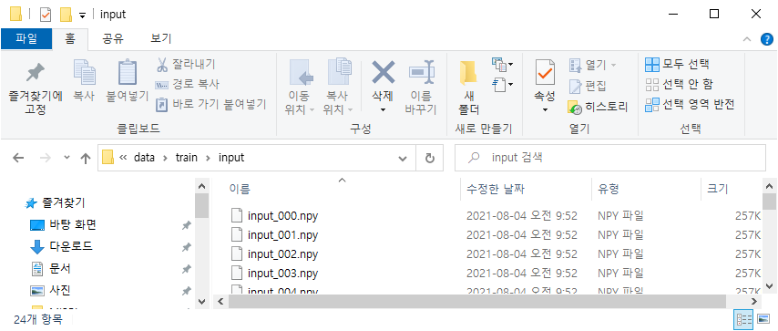
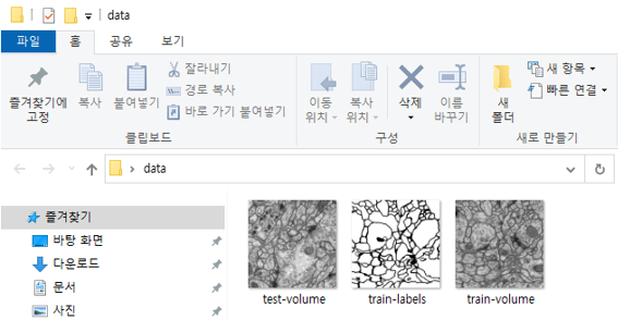
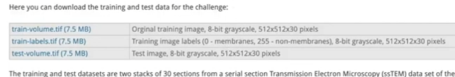
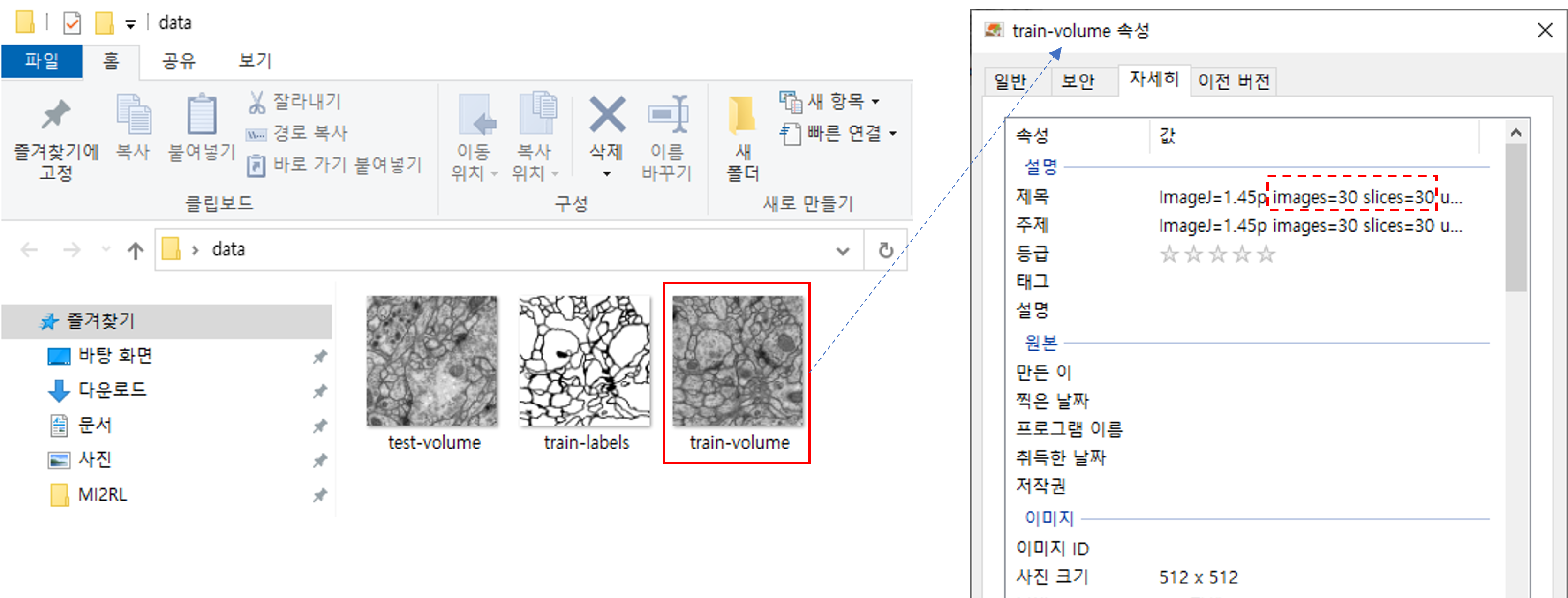
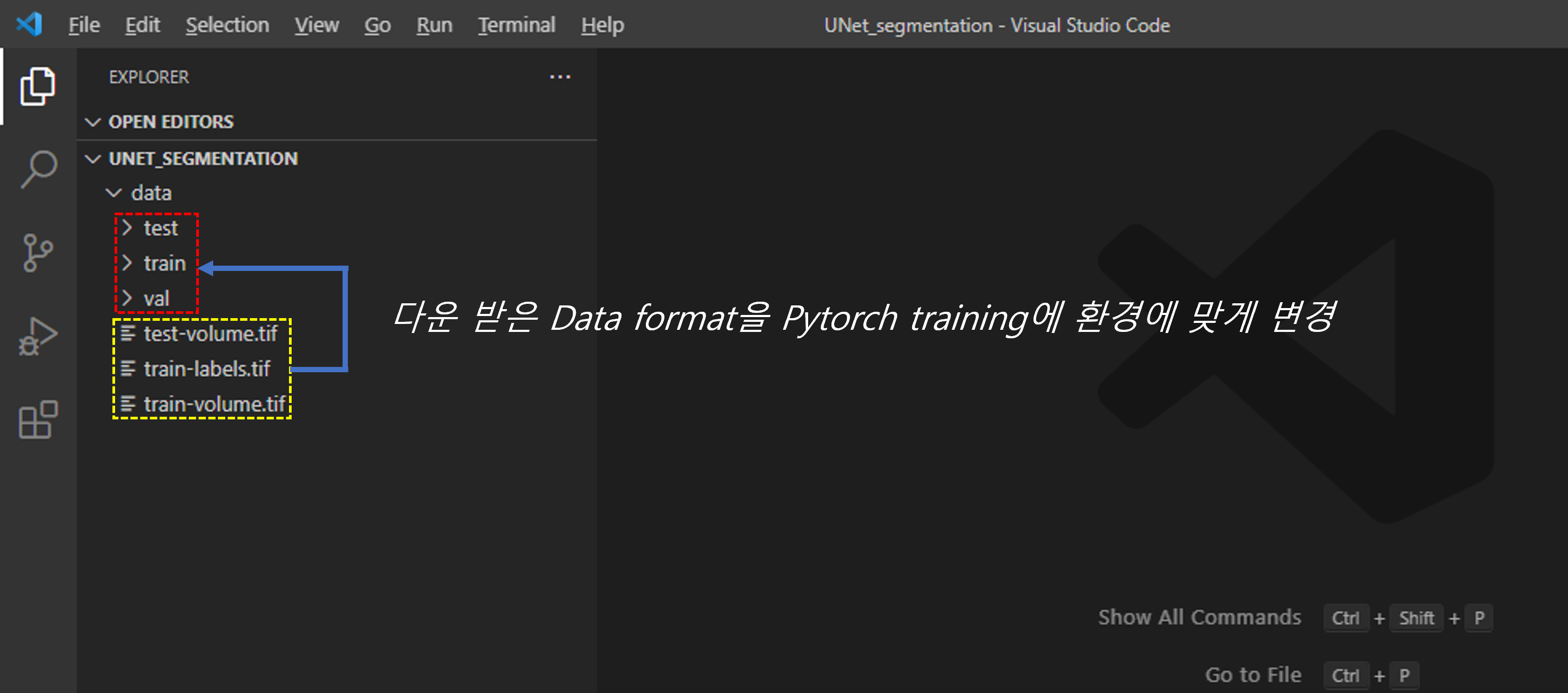
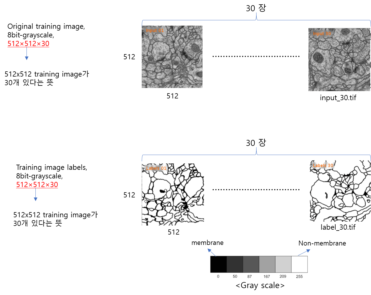
예를 들어, 아래 train-labels 이미지 정보를 보면 512×512×30 형태로 제공된 것을 볼 수 있습니다.

512×512×30에서 30이 의미하는 바는 특정 이미지 frame을 의미합니다. 예를 들어, (512, 512, 1) 값들은 첫 번째 이미지frame을 뜻하고, (512, 512, 2) 값들은 두 번 째 이미지 frame을 뜻합니다.

그래서 위와 같은 이미지 형태를 읽어들일 때는 frame 단위로 이미지를 읽어야 하는 경우가 있습니다.이러한 경우는 seek 이라는 함수를 이용합니다.

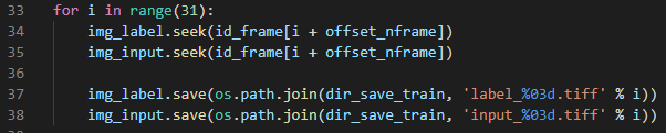
for문과 seek() 함수를 통해 frame 별 이미지들을 하나씩 따로 불러올 수 있습니다.

이렇게 불러온 binary mode 이미지를 0~255 값으로, 즉 사람이 읽을 수 있는 값으로 변형 시키려면 numpy 패키지에서 제공해주는 함수를 이용하면 됩니다. 아래 코드에서는 numpy.asarray() 함수를 이용했네요.

굳이 위와 같이 numpy로 변경 시켜줄 필요 없이, tiff 이미지만 저장시키고 싶은 경우는 아래와 같이 코드를 작성해주면 됩니다.

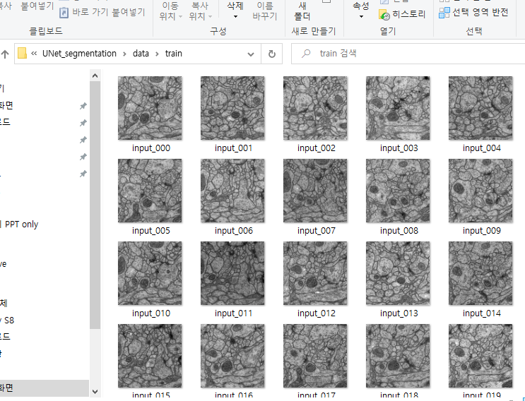
그럼 아래와 같이 이미지가 frame 별로 따로 'tiff' 형식으로 저장되는걸 확인하실 수 있습니다.

지금까지 Image 모듈에 대한 설명과 기본적인 함수인 Image.open(), Image.seek() 에 대해서 알아보았습니다.

감사합니다.

안녕하세요.

이번 글에서는 Pillow라는 파이썬 패키지에 대해서 소개해드리려고 합니다.

1. Pillow 패키지란?

Pillow 패키지를 설명하기 전에 PIL 패키지에 대해 간단히 설명하겠습니다.

PIL는 Python Imaging Libarary의 약자로, 파이썬으로 이미지를 다룰 때 유용한 기능들을 제공하는 라이브러리 였습니다.

"PIL is the Python Imaging Library by Fredrik Lundh and Contributors."

파이썬에서 setuptools이란 python 라이브러리 를 확장 및 배포하는데  사용되는 extension libarary인데, 이러한 setuptools을 이용하여 프로젝트 빌드, 배포를 쉽게 관리할 수 있게 도와줍니다. 하지만, PIL는 "not setuptools compatible" 하다고 알려져 있었기 때문에 이를 개선하고자 PIL를 fork하여 Pillow라는 프로젝트를 실행하게 됩니다. (파이썬에 이미지를 다루는 또 다른 패키지로는 openCV가 있습니다)

(↓↓↓Pillow 공식 사이트↓↓↓)

https://pillow.readthedocs.io/en/stable/

2. Pillow 패키지 설치하는 방식은?

Pillow 패키지를 설치하기 전에 알아두어야 할 사항들을 정리해보겠습니다.

2-1. PIL 설치 여부 확인

Pillow를 설치하는 방법을 알려주는 사이트에 접속하면 아래와 같은 주의사항을 알려줍니다.

"Pillow and PIL cannot co-exist in the same environment. Before installing Pillow, please uninstall PIL."

즉, Pillow를 설치하기 전에 PIL가 있으면, PIL를 uninstall 해주어야 합니다.

(↓↓↓Pillow 설치 방식↓↓↓)

https://pillow.readthedocs.io/en/stable/installation.html#warnings

2-2. Python 버전 확인

지금까지 Pillow 패키지는 여러 업데이트를 통해 다양한 버전이 release 되었습니다. 

Python 패키지도 마찬가지로 다양한 버전이 있죠.

그래서, Pillow 패키지를 설치 할 시, 파이썬 버전과 Pillow 패키지 간의 호환성을 고려해야 합니다.

(예를 들어, Pillow 7.0 버전을 만들 때는 python 3.5 버전의 기능 중 python 3.4에서 추가된 기능등을 이용했다고 하면, 당연히 python 3.4 버전에서는 호환이 안되겠죠?)

2-3. OS (Operating System) 확인

사실 패키지를 설치하기 위해서 OS까지 확인하는 경우는 없지만, 만일의 경우에 대비해서 Pillow 개발자들이 테스트한 환경에 맞게 세팅해준다면 더 안전할 수 있겠죠?

아래와 같은 표를 보면 OS 마다 Pillow를 어떤 python 버전에서 테스트 했는지 나와있습니다. 

Supporting해주는 python 버전이 있으니, python 버전에 맞는 Pillow 패키지 버전을 설치해주면 되겠죠? 

(Tested architecture 부분은 CPU 모델과 관련된 설명인데, 자세한 부분은 아래 글을 참고해주세요)

https://89douner.tistory.com/151

2-5. Pillow 패키지 설치

아래와 같은 명령어를 사용하시면 Pillow 패키지가 설치 됩니다.

python3 -m pip install --upgrade pip
python3 -m pip install --upgrade Pillow

하지만, 아나콘다 가상환경을 이용하시는 분은 Pillow 패키지 설치 시, 아래의 글을 참고해주세요! 

("ctrl+F" 누른 후, "pillow" 검색)

https://89douner.tistory.com/73

3. Pillow 모듈

Pillow 패키지에는 굉장히 다양힌 모듈들이 있습니다.

어떠한 이미지 관련 기능을 제공해주는지에 따라서 모듈의 종류가 결정됩니다.

(↓↓↓Pillow 모듈들 reference↓↓↓)

https://pillow.readthedocs.io/en/stable/reference/index.html

※참고로 파이썬에서 모듈이란 "함수나 변수 또는 클래스를 모아 놓은 파일"을 지칭합니다.

(↓↓↓모듈에 대한 설명↓↓↓)

https://wikidocs.net/29

그렇다면, Pillow 패키지 중 가장 기본이 되는 Image 모듈에는 어떤 기능이 있을까요?

이러한 모듈을 어떻게 사용할 수 있을까요?

다음 글에서 알아보도록 하겠습니다!

안녕하세요.

이번 글에서는 CNN 모델의 학습할 방향성을 정해주기 위한 loss function, opimizer, learning rate policy를 설정해주는 코드들을 살펴보도록 하겠습니다.

import torch.nn as nn
import torch.optim as optim
from torch.optim import lr_scheduler

1. Loss function 설정

torch.nn 을 살펴보면 다양한 neural network를 제공해주는 것 외에 loss function도 제공해주고 있다는 걸 확인할 수 있습니다.

https://pytorch.org/docs/stable/nn.html

CNN 학습을 위해 torch.nn에서 제공해주는 CrossEntropyLoss를 사용합니다. (다른 loss function도 사용가능 하지만 보통은 crossentropy loss를 사용합니다)

2. optimizer 정의 (Feat. 최신 optimizer 사용방식)

torch.optim 이라는 패키지를 살펴보면 다양한 optimizer를 제공해준다는 것을 알 수 있습니다.

(경험상 optimizer를 무엇으로 사용했는지에 따라 딥러닝 모델 성능에 많은 영향을 끼치는걸 확인할 수 있었기 때문에 어떠한 optimizer를 사용할지 잘 결정하는 것이 중요합니다.)

https://pytorch.org/docs/stable/optim.html

(↓↓↓optimizer 관련 내용 정리한 글↓↓↓)

https://89douner.tistory.com/46

torch.optim은 가장 기본이 되는 optimizer들을 제공합니다.

하지만 최신 SOTA 성능의 optimizer들은 제공하지 않는 경우가 많죠.

그래서 SOTA 성능의 optimizer를 이용하기 위해서는 다른 방법을 찾아야 합니다.

보통 SOTA optimizer 같은 경우는 논문으로 출판할 때, 해당 optimizer를 이용할 수 있게 github에 업로드합니다. 업로드된 optimizer를 패키지로 다운받아 pytorch, tensorflow와 연동해서 사용하면 됩니다.

예를 들어, adabelief optimizer라는 최신 optimizer가 나왔다고 하면 아래와 같은 순서를 따라 이용하면 됩니다.

1) adabelief optimizer github 사이트 검색

https://github.com/juntang-zhuang/Adabelief-Optimizer

 2) 위의 사이트에서 언급한대로 adabelief optimizer 패키지 설치

• 여기에서는 pytorch 버전 설치
• 다른 가상환경을 사용하고 있으면 해당 가상환경에 설치하는데 필요한 명령어로 바꾸어 설치 (ex: anaconda)

pip install adabelief-pytorch==0.2.0

 3) 설치한 adabelief optimizer 패키지 설치 후, 해당 optimizer 이용

from adabelief_pytorch import AdaBelief
optimizer_ft = AdaBelief(model.parameters(), lr=1e-3, eps=1e-16, betas=(0.9,0.999), weight_decouple = True, rectify = False)

3. learning rate scheduler (policy) 정의

앞서 optimizer를 정의 했다면, learning rate policy를 정해주어야 합니다.

기본적인 learning rate policy 역시 torch.opim에서 제공해주니 아래 API를 참고하시면 다양한 learning rate policty를 확인하실 수 있습니다.

https://pytorch.org/docs/stable/optim.html

Learning rate policy는 정말 다양하게 있는데 대표적인 경우들에 대해서 소개하도록 하겠습니다.

1) Step policy

학습을 하다보면 loss가 정체되어 있는 경우가 있습니다. 이 경우 early stoping을 하여 학습을 종료시키는 경우도 있지만 아래 "그림10"에서 처럼 정체되는 순간 learning rate을 감소시켜주면 loss가 다시 줄어드는경우도 있습니다. 

이와 같이 계단 형식으로 learning rate을 감소(decay) 시켜주는 learning rate policy 방식을 step decay라고 합니다.

Step decay 방식을 이요하려면 아래와 같이 코드를 작성해주면 됩니다.

아래와 같은 코드를 작성해주면 3번의 epoch 마다 learning rate가 0.1씩 감소하게 됩니다. 

(↓↓↓pytorch에서 제공해주는 step learning rate policy API↓↓↓)

https://pytorch.org/docs/stable/generated/torch.optim.lr_scheduler.StepLR.html#torch.optim.lr_scheduler.StepLR

2) Cosine annealing policy

Pytorch에서는 step learning rate policy외에 cosine annealing policy라는 방식도 제공해줍니다. 

보통은 cosine annealing policy를 warm_up과 같이 사용하는데, 이에 대해서는 뒷 부분에서 설명하도록 하겠습니다.

• optimizer – Wrapped optimizer.
• T_max (int)  – Maximum number of iterations.
• eta_min (float)  – Minimum learning rate. Default: 0.
• last_epoch (int) – The index of last epoch. Default: -1.

(↓↓↓pytorch에서 제공해주는 Cosine Annealing learning rate policy API↓↓↓)

https://pytorch.org/docs/stable/generated/torch.optim.lr_scheduler.CosineAnnealingLR.html#torch.optim.lr_scheduler.CosineAnnealingLR

3) Warm_up policy

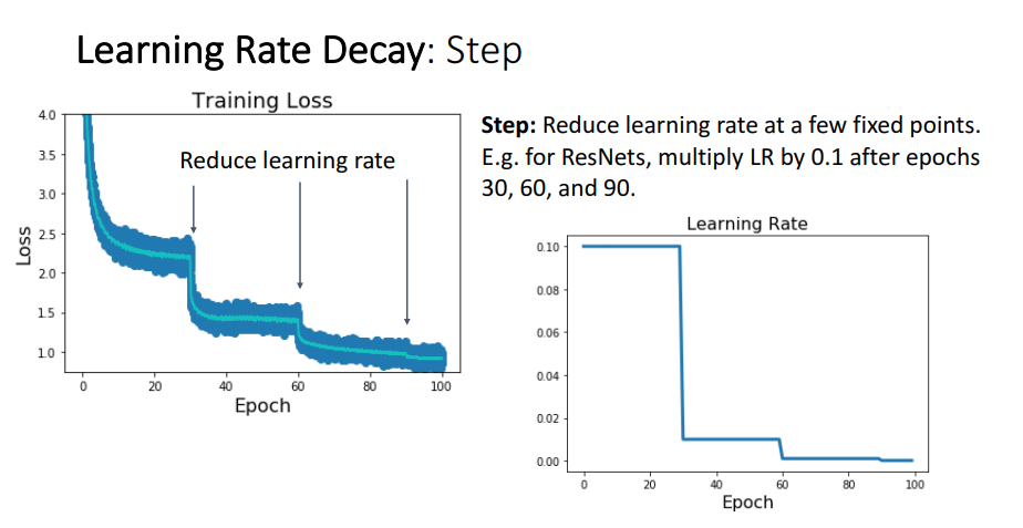
초기에는 layer 값들이 굉장히 불안정하기 때문에 너무 큰 learning rate을 적용하면 loss값이 지나치게 커질 수 있습니다. 그래서 초기의 unstable 상태를 고려해 초기 특정 epoch 까지는 learning rate을 천천히 증가시켜주는 방식이 warm_up 방식입니다.

Warm_up을 통해 특정 epoch 까지 learning rate을 증가시키면, 특정 epoch 이후에는 기존 learning rate policy를 적용시켜주어야 합니다. 

아래 그림을 보면 초기 5 epoch 까지는 learning rate을 점진적으로 증가시키고, 5 epoch 이후에는 step policy 또는 cosine annealing policy  확인할 수 있습니다.

Warm_up policy는 pytorch에서 기본 learning rate policy로 제공해주고 있지 않기 때문에 따로 warm_up laerning rate policy 패키지를 설치해야합니다.

3-1) Warm_up policy with step learning rate policy

3-1-1) warm_up step learning rate과 관련된 사이트 검색 

https://github.com/ildoonet/pytorch-gradual-warmup-lr

3-1-2) 패키지 설치

pip install git+https://github.com/ildoonet/pytorch-gradual-warmup-lr.git

3-1-3) 설치된 패키지 이용

criterion = nn.CrossEntropyLoss()

# Observe that all parameters are being optimized
optimizer_ft = optim.SGD(model_ft.parameters(), lr=0.001, momentum=0.9) 

# Decay LR by a factor of 0.1 every 3 epochs
exp_lr_scheduler = lr_scheduler.StepLR(optimizer_ft, step_size=3, gamma=0.1)
exp_lr_scheduler = GradualWarmupScheduler(optimizer_ft, multiplier=1, total_epoch=5, after_scheduler=exp_lr_scheduler)

3-2) Warm_up policy with cosine annealing learning rate policy

3-2-1) warm_up consine annealing learning rate과 관련된 사이트 검색 

https://github.com/katsura-jp/pytorch-cosine-annealing-with-warmup

3-2-2) 패키지 설치

pip install 'git+https://github.com/katsura-jp/pytorch-cosine-annealing-with-warmup'

3-2-3) 설치된 패키지 이용

from cosine_annealing_warmup import CosineAnnealingWarmupRestarts

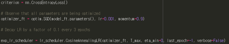
criterion = nn.CrossEntropyLoss()
optimizer_ft = optim.SGD(model.parameters(), lr=0.1, momentum=0.9, weight_decay=1e-5) # lr is min lr
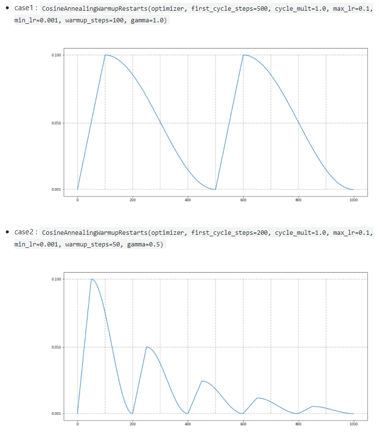
scheduler = CosineAnnealingWarmupRestarts(optimizer, first_cycle_steps=200, cycle_mult=1.0, max_lr=0.1, min_lr=0.001, warmup_steps=50, gamma=1.0)

Cosine annealing with warm_up 과 관련된 hyper parameter들은 아래 그림을 보면 이해하시기 편하실 겁니다. (참고로 gamma부분은 다음 cycle에서 max_lr을 어느 정도 줄여줄지를 결정해주는 hyper parameter 입니다)

Warm_up을 적용시킬 때 batch size에 따라 initial learning rate(=마지막 warm up 단계에서의 learning rate)를 어떻게 설정해 줄 지 결정해 주기도 합니다. 이 부분은 아래 글에서 learning rate warmup 부분을 참고해주시면 될 것 같습니다.

https://89douner.tistory.com/248

4. 요약

지금까지 배운 내용을 잠시 정리 해보겠습니다.

# License: BSD
# Author: Sasank Chilamkurthy

from __future__ import print_function, division

import torch
import torch.nn as nn
import torch.optim as optim
from torch.optim import lr_scheduler
import numpy as np
import torchvision
from torchvision import datasets, models, transforms
import matplotlib.pyplot as plt
import time
import os
import copy

plt.ion()   # interactive mode

4-1. Data Load

먼저 아래 글을 통해 CNN 학습을 위하 이미지 데이터들을 어떻게 load 하는지에 대해서 설명했습니다.

https://89douner.tistory.com/287?category=994842 

# Data augmentation and normalization for training
# Just normalization for validation
data_transforms = {
    'train': transforms.Compose([
        transforms.RandomResizedCrop(224),
        transforms.RandomHorizontalFlip(),
        transforms.ToTensor(),
        transforms.Normalize([0.485, 0.456, 0.406], [0.229, 0.224, 0.225])
    ]),
    'val': transforms.Compose([
        transforms.Resize(256),
        transforms.CenterCrop(224),
        transforms.ToTensor(),
        transforms.Normalize([0.485, 0.456, 0.406], [0.229, 0.224, 0.225])
    ]),
}

data_dir = 'data/hymenoptera_data'
image_datasets = {x: datasets.ImageFolder(os.path.join(data_dir, x),
                                          data_transforms[x])
                  for x in ['train', 'val']}
dataloaders = {x: torch.utils.data.DataLoader(image_datasets[x], batch_size=4,
                                             shuffle=True, num_workers=4)
              for x in ['train', 'val']}
dataset_sizes = {x: len(image_datasets[x]) for x in ['train', 'val']}
class_names = image_datasets['train'].classes

device = torch.device("cuda:0" if torch.cuda.is_available() else "cpu")

추가적으로 batch 단위로 augmentation이 적용된 이미지 데이터들을 아래 함수로 확인해볼 수 있었습니다.

def imshow(inp, title=None):
    """Imshow for Tensor."""
    inp = inp.numpy().transpose((1, 2, 0))
    mean = np.array([0.485, 0.456, 0.406])
    std = np.array([0.229, 0.224, 0.225])
    inp = std * inp + mean
    inp = np.clip(inp, 0, 1)
    plt.imshow(inp)
    if title is not None:
        plt.title(title)
    plt.pause(0.001)  # pause a bit so that plots are updated


# Get a batch of training data
inputs, classes = next(iter(dataloaders['train']))

# Make a grid from batch
out = torchvision.utils.make_grid(inputs)

imshow(out, title=[class_names[x] for x in classes])

4-2. Data Preprocessing

아래 글을 통해 학습 데이터를 전처리하기 위한 다양한 방식들에 대해서 다루어 봤습니다.

(작성중....)

4-3.  CNN

CNN 모델(ResNet)을 처음부터 scratch로 구현해보았습니다.

https://89douner.tistory.com/288?category=994842 

4-4.  Transfer Learning (Feat. Pre-trained model, GPU)

pre-trained model을 다운 받아 transfer learning을 적용하는 코드에 대해서 다루었고, 추가적으로 해당 모델을 GPU에 업로드 하는 것 까지 살펴봤습니다.

https://89douner.tistory.com/289?category=994842 

model_ft = models.resnet18(pretrained=True)
num_ftrs = model_ft.fc.in_features
# Here the size of each output sample is set to 2.
# Alternatively, it can be generalized to nn.Linear(num_ftrs, len(class_names)).
model_ft.fc = nn.Linear(num_ftrs, 2)

model_ft = model_ft.to(device)

4-5.  Loss function, Optimizer, Learning rate policy (← 현재 글)

이번 글에서는 딥러닝 모델이 학습할 방향성에 대해서 정리했고, 관련 코드는 아래와 같습니다.

criterion = nn.CrossEntropyLoss()

# Observe that all parameters are being optimized
optimizer_ft = optim.SGD(model_ft.parameters(), lr=0.001, momentum=0.9)

# Decay LR by a factor of 0.1 every 7 epochs
exp_lr_scheduler = lr_scheduler.StepLR(optimizer_ft, step_size=7, gamma=0.1)

5. 코드 정리

지금까지 배운 내용을 코드로 정리하면 아래와 같습니다.

# License: BSD
# Author: Sasank Chilamkurthy

from __future__ import print_function, division

import torch
import torch.nn as nn
import torch.optim as optim
from torch.optim import lr_scheduler
import numpy as np
import torchvision
from torchvision import datasets, models, transforms
import matplotlib.pyplot as plt
import time
import os
import copy
from warmup_scheduler import GradualWarmupScheduler

plt.ion()   # interactive mode

# Data augmentation and normalization for training
# Just normalization for validation
data_transforms = {
    'train': transforms.Compose([
        transforms.RandomResizedCrop(224),
        transforms.RandomHorizontalFlip(),
        transforms.ToTensor(),
        transforms.Normalize([0.485, 0.456, 0.406], [0.229, 0.224, 0.225])
    ]),
    'val': transforms.Compose([
        transforms.Resize(256),
        transforms.CenterCrop(224),
        transforms.ToTensor(),
        transforms.Normalize([0.485, 0.456, 0.406], [0.229, 0.224, 0.225])
    ]),
}

data_dir = 'data/hymenoptera_data'
image_datasets = {x: datasets.ImageFolder(os.path.join(data_dir, x),
                                          data_transforms[x])
                  for x in ['train', 'val']}
dataloaders = {x: torch.utils.data.DataLoader(image_datasets[x], batch_size=4,
                                             shuffle=True, num_workers=4)
              for x in ['train', 'val']}
dataset_sizes = {x: len(image_datasets[x]) for x in ['train', 'val']}
class_names = image_datasets['train'].classes

device = torch.device("cuda:0" if torch.cuda.is_available() else "cpu")

def imshow(inp, title=None):
    """Imshow for Tensor."""
    inp = inp.numpy().transpose((1, 2, 0))
    mean = np.array([0.485, 0.456, 0.406])
    std = np.array([0.229, 0.224, 0.225])
    inp = std * inp + mean
    inp = np.clip(inp, 0, 1)
    plt.imshow(inp)
    if title is not None:
        plt.title(title)
    plt.pause(0.001)  # pause a bit so that plots are updated


# Get a batch of training data
inputs, classes = next(iter(dataloaders['train']))

# Make a grid from batch
out = torchvision.utils.make_grid(inputs)

imshow(out, title=[class_names[x] for x in classes])

model_ft = models.resnet18(pretrained=True)
num_ftrs = model_ft.fc.in_features
# Here the size of each output sample is set to 2.
# Alternatively, it can be generalized to nn.Linear(num_ftrs, len(class_names)).
model_ft.fc = nn.Linear(num_ftrs, 2)

model_ft = model_ft.to(device)

criterion = nn.CrossEntropyLoss()

# Observe that all parameters are being optimized
optimizer_ft = optim.SGD(model_ft.parameters(), lr=0.001, momentum=0.9) 

# Decay LR by a factor of 0.1 every 3 epochs
exp_lr_scheduler = lr_scheduler.StepLR(optimizer_ft, step_size=3, gamma=0.1)
exp_lr_scheduler = GradualWarmupScheduler(optimizer_ft, multiplier=1, total_epoch=5, after_scheduler=exp_lr_scheduler)

6. 다음 글에서 배울 내용

지금까지 딥러닝 학습을 위한 모든 준비를 끝냈습니다.

그렇다면 딥러닝이 실제로 어떤 단계(code)를 통해 학습하는지 알아봐야겠죠?

이 부분에 대한 내용은 train_model이라는 함수를 통해 실행이 되는데 이 부분은 다음 글에서 살펴보도록 하겠습니다.

(↓↓↓다음 글에서 배울 코드↓↓↓) 

model_ft = train_model(model_ft, criterion, optimizer_ft, exp_lr_scheduler, num_epochs=20)

안녕하세요.

이번 글에서는 transfer learning을 pytorch로 적용하는 방법에 대해서 알아보도록 하겠습니다. 

CNN 모델을 training하는 방식에는 2가지가 있습니다.

1. Scratch training (learning)
   • 자신의 데이터 셋을 기반으로 CNN 모델을 구현하여 학습시키는 방법
   • Scratch training을 하려는 경우에는 지난 글("3.CNN 구현")에서 설명한 방식대로 CNN 모델을 구현하고 자신의 데이터셋을 학습시키면 됩니다. 
2. Transfer learning (← 이번 글에서 설명)
   • ImageNet과 같은 데이터셋으로 학습시킨 CNN 모델을 pre-train 모델이라고 합니다.
   • Transfer learning은 이러한 pre-train 모델을 이용합니다.
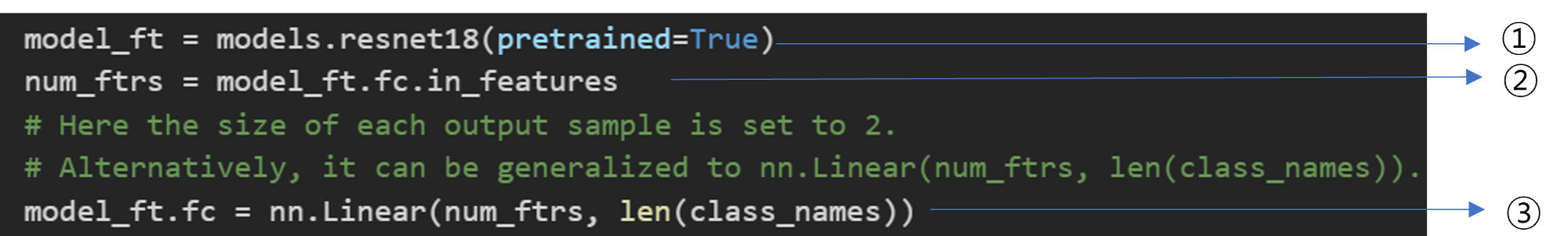
   • Pre-trained 모델은 FC layer의 마지막 뉴런 수(=ImageNet 클래스 개수)가 1000 입니다. 그래서, 나의 task가 3개의 class를 분류해야하는 것이라면 FC layer의 마지막 뉴런 수가 3개인 FC layer로 교체해줘야 합니다. (← 자세한 설명은 뒤에서)

그럼 지금부터 transfer learning 적용을 위한 아래 코드들을 하나씩 설명해보도록 하겠습니다.

1. Pre-trained model 다운받기

from torchvision import models

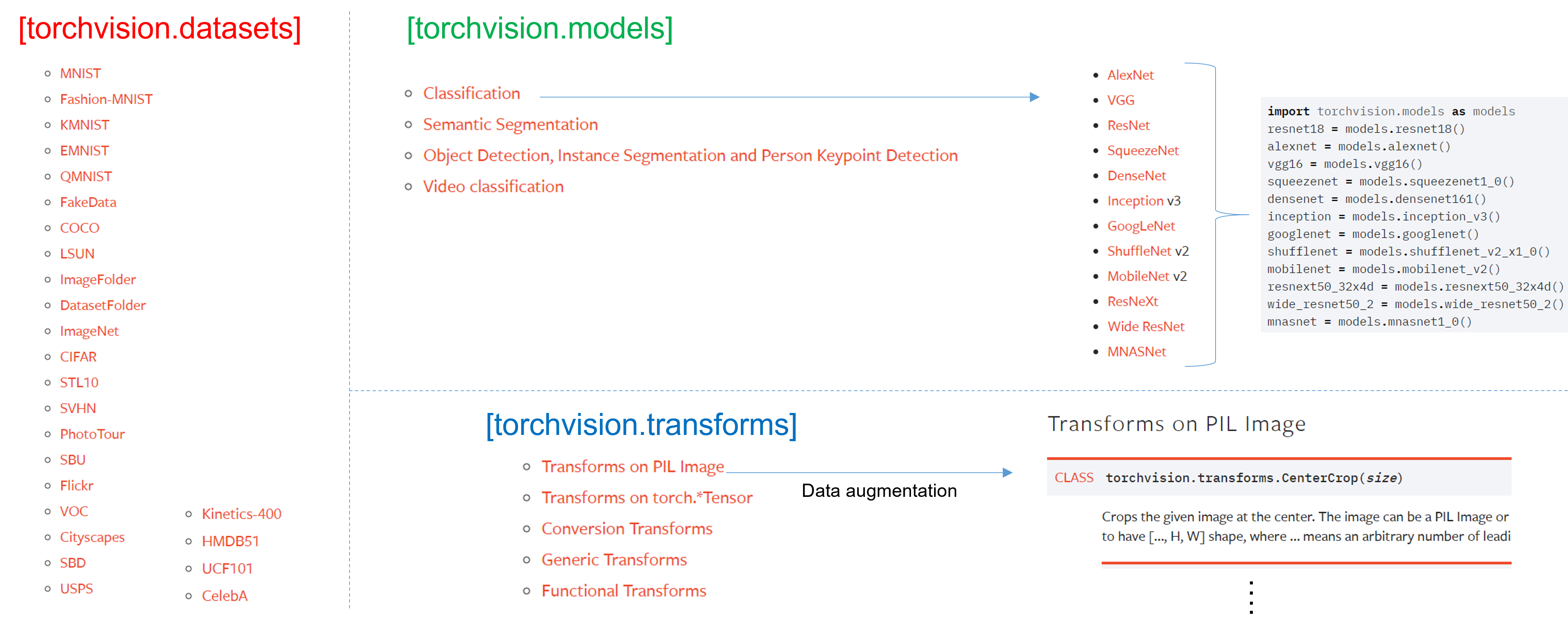
앞선 글("1.Data Load(Feat. CUDA)")에서 torchvision이 크게 3가지 기능을 제공한다고 언급했고, 이 중 2가지인 transforms와 datasets에 대해서 설명드린바 있습니다. 

이번 글에서는 torchvision의 또 다른 기능인 models에 대해 설명드리도록 하겠습니다.

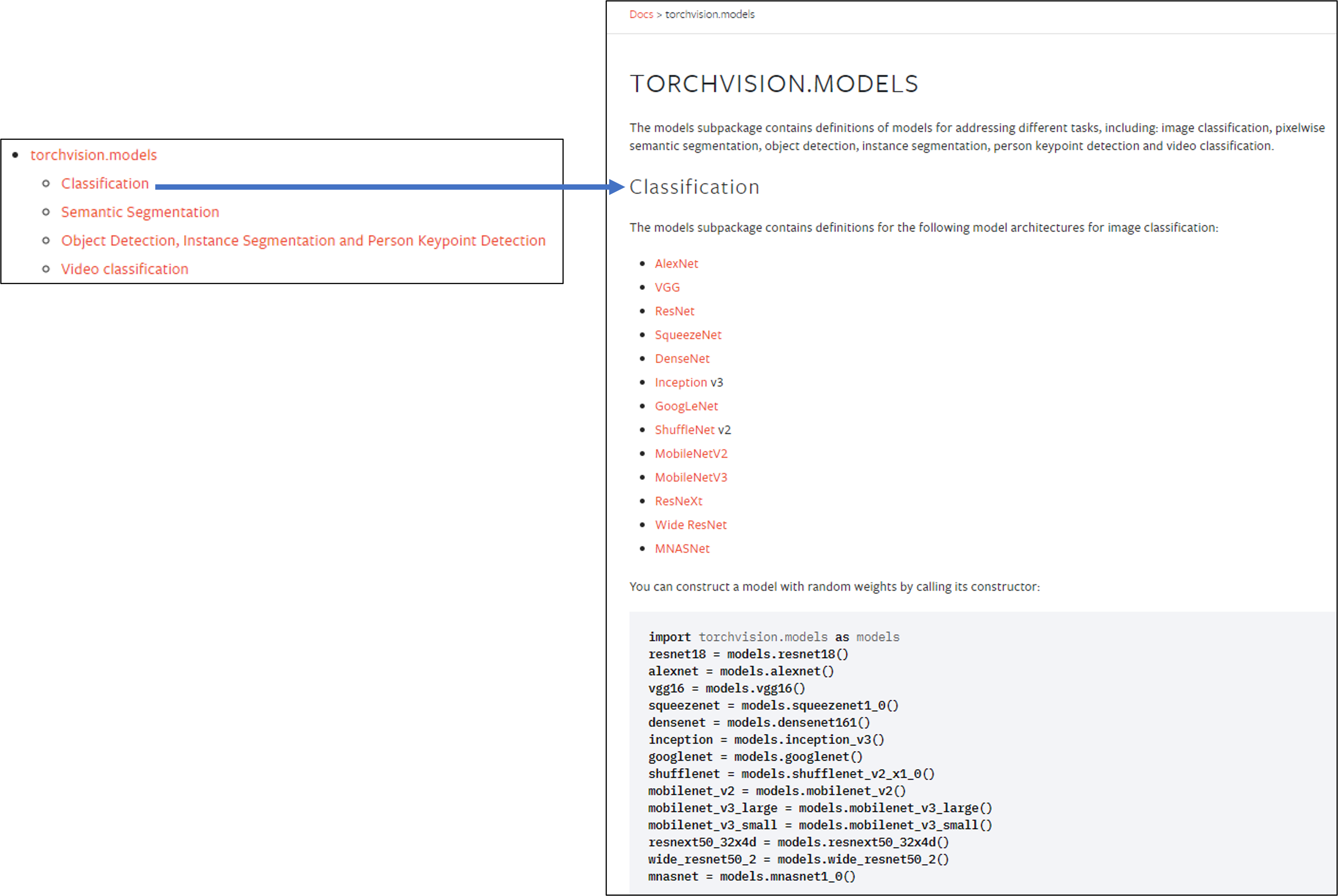
torchvision.models 패키지는 다양한 이미지 task 분야 (ex: classification, dobject detection, segmentation, etc)의 pre-trained 모델을 제공해주고 있습니다.

(↓↓↓classification pre-trained model을 제공해주는 torchvision↓↓↓)

https://pytorch.org/vision/stable/models.html#classification

아래 코드를 입력하면 pre-trained model이 다운받아집니다.

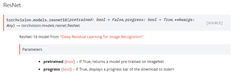
아래 parameters를 보면 알 수 있듯이 pre-trained model은 ImageNet을 기반으로 하고 있는걸 확인할 수 있습니다. 만약 "pretrained=False"로 설정하면 resnet18 모델만 사용할 수 있게 됩니다 (=Conv filter가 학습이 되지 않은 초기화 상태)

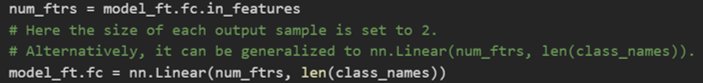
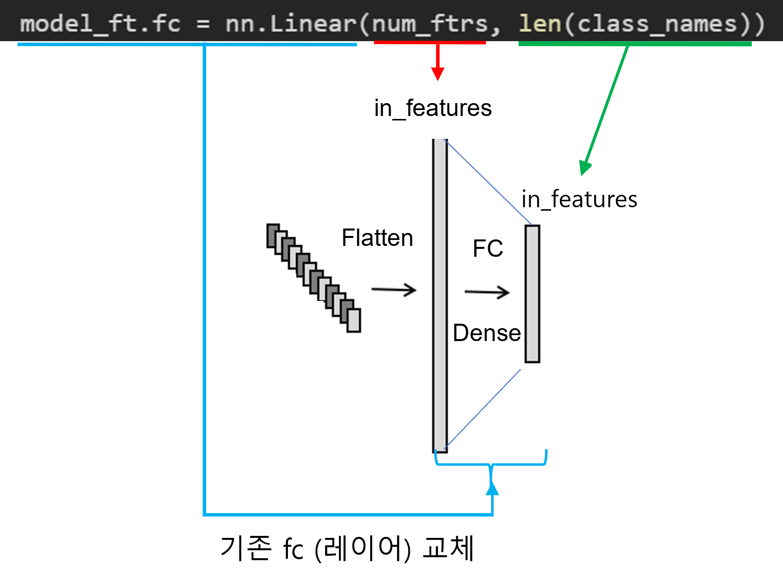
2. FC layer 수정해주기

앞서 Pre-trained model을 다운 받았으니 내가 사용할 task에 맞게 FC layer를 변경해주어야 합니다.

import torch.nn as nn

num_ftrs 가 의미하는 바는 아래와 같습니다.

(↓↓↓ResNet 구현된 API↓↓↓)

https://pytorch.org/vision/stable/_modules/torchvision/models/resnet.html#resnet18

"1.Data Load (Feat.CUDA)" 글에서 class_names는 폴더에 있는 클래스 명들을 담고 있다고 했습니다. 만약 분류해야할 클래스가 5개이면 해당 폴더도 5가지로 구성되어 있으니, len(class_name)을 적용하면 5라는 값이 출력 될 것입니다.

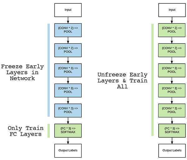
3. Fine-tuning 정도 정해주기 (Feat. freezing)

Transfer learning을 적용할 때 상황에 따라 어느 layer까지 학습 가능하게 할지 고려해주어야 합니다.

(↓↓↓Transfer learning을 적용할 때 고려해야할 상황 4가지↓↓↓)

https://89douner.tistory.com/67

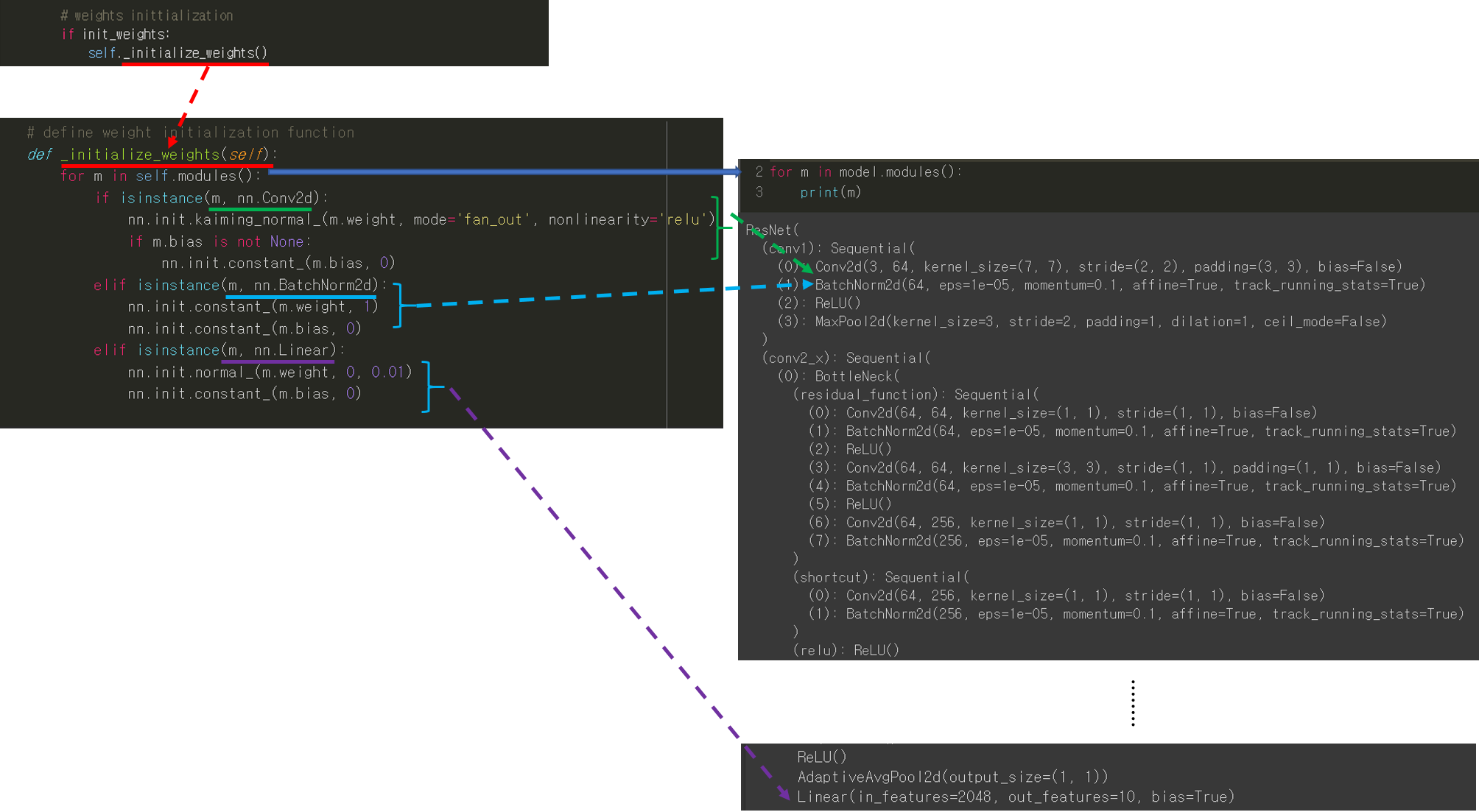
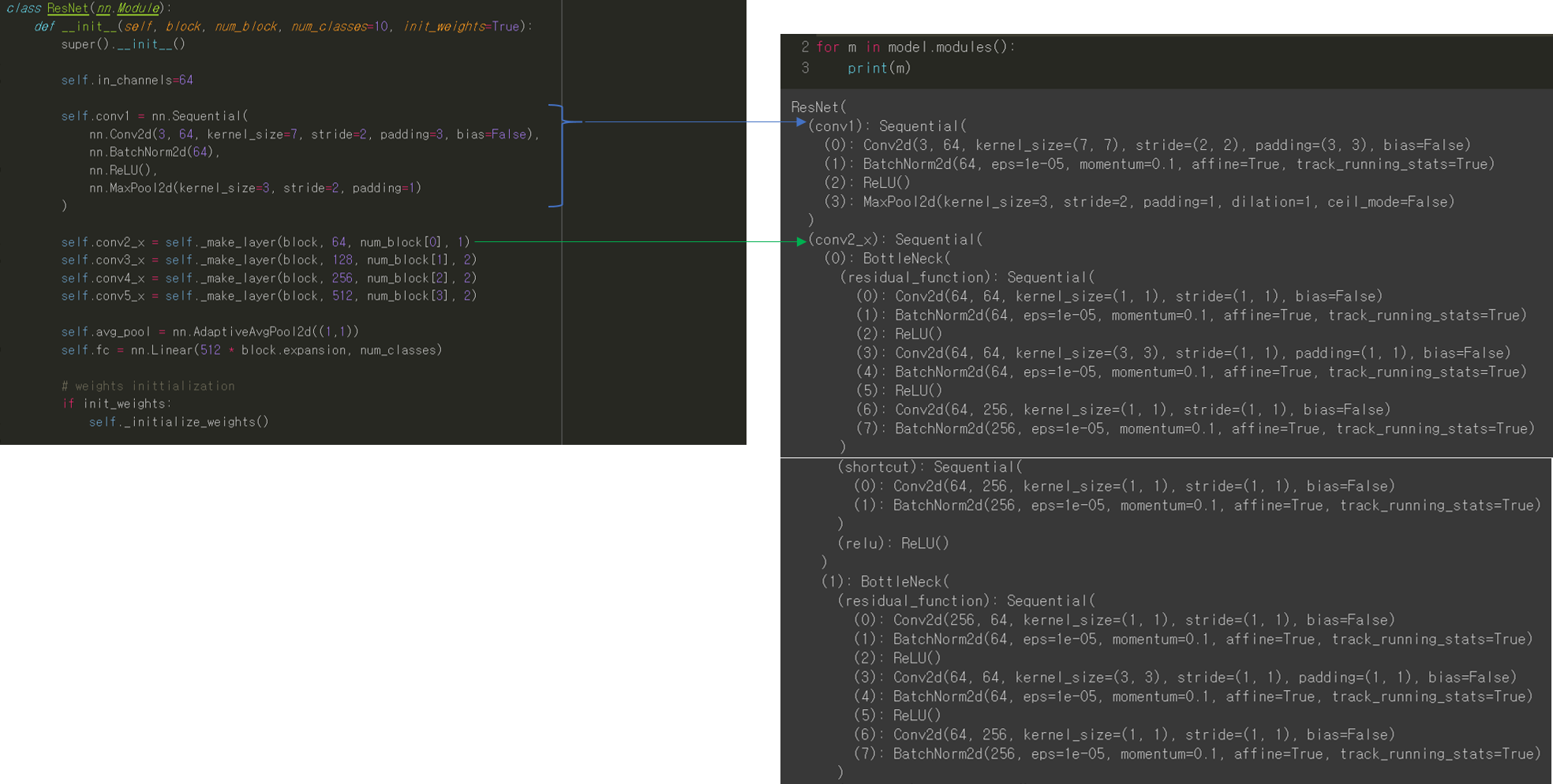
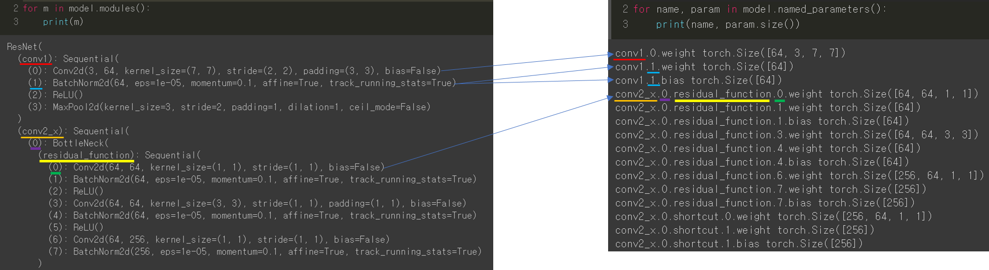
Freezing 정도를 pytorch에서는 어떻게 설정해주는지 글로 쓰려고 했는데, 따로 정리한 PPT에 설명이 잘되어 있어서 아래 PPT 자료로 설명을 대체하겠습니다. (파일 용량이 10MB 이상 업로드가 안돼서 디자인도 바꾸고 중간중간 슬라이드 부분도 제거해버렸네요 ㅜㅜ)

또한 특정 layer의 conv filter 또는 batch normalization의 beta, gamma 값을 초기화(initialization) 해주어야 할 때도 있습니다. 이러한 경우 어떻게 초기화 시키면 되는지 또한 PPT 자료로 정리해놨으니 참고해주시면 감사하겠습니다 (파일 용량이 10MB 이상 업로드가 안돼서 디자인도 바꾸고 중간중간 슬라이드 부분도 제거해버렸네요 ㅜㅜ)

(↓↓↓batch norm gamma, beta 초기화 필요성을 언급한 논문↓↓↓)

https://89douner.tistory.com/248?category=908624 

3. Model을 GPU에 업로드 하기

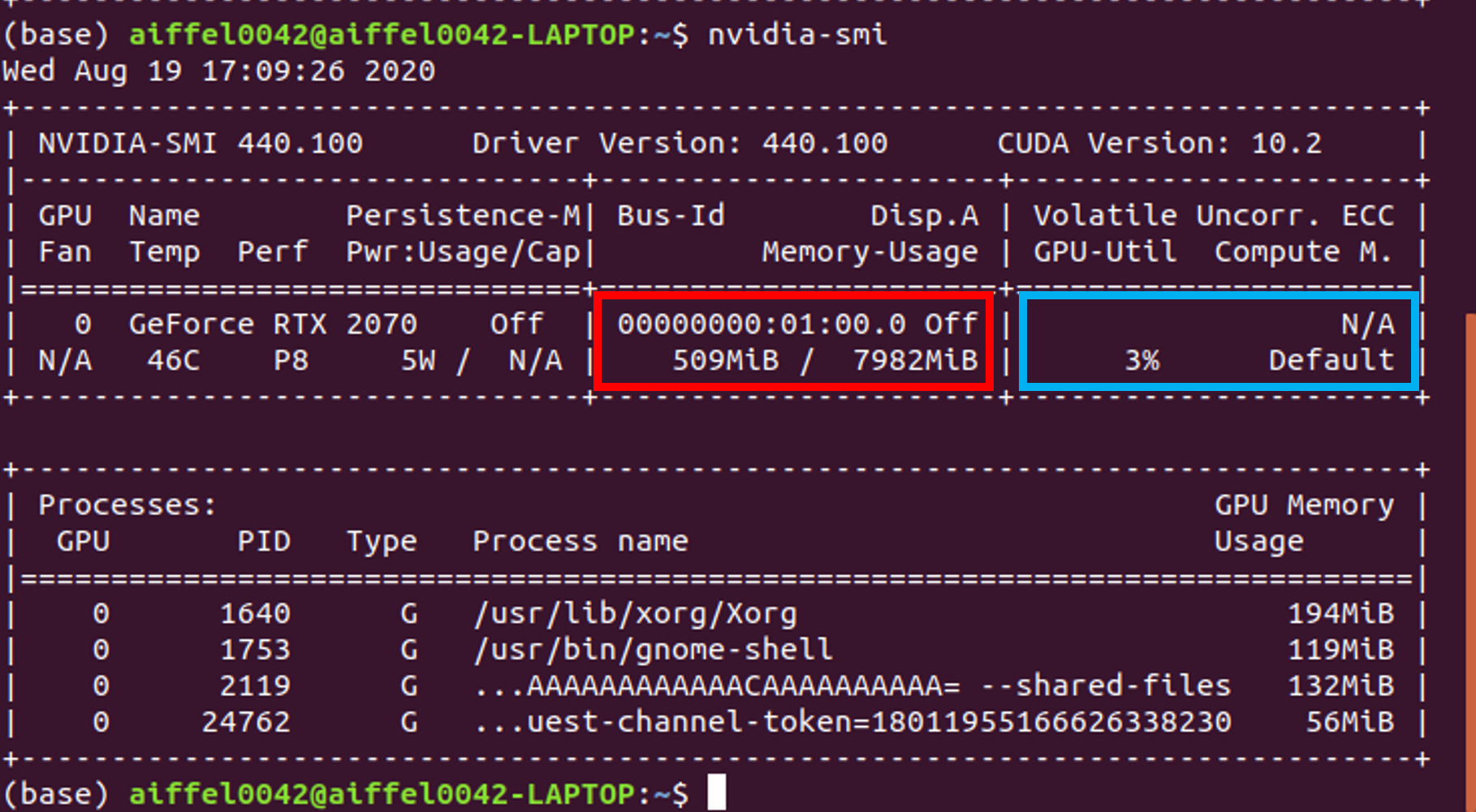
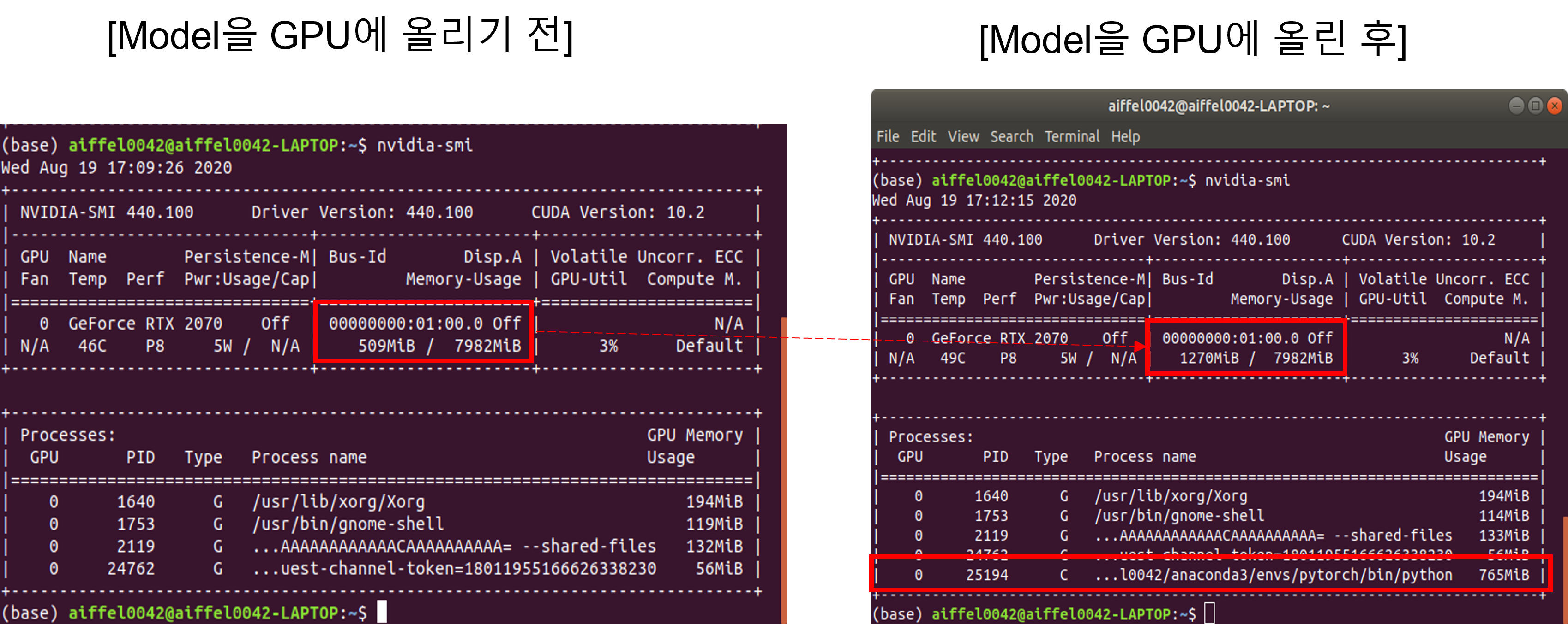
학습하기 위해 모델 구축을 마무리 했습니다. 그럼 실제 학습을 위해 이제부터 딥러닝 model을 GPU에 올려놓도록 하겠습니다.

아직 model을  GPU에 올리기 전 상태이기 때문에, nvidia-smi를 통해 GPU 메모리를 확인하면 대략 500MiB의 메모리가 다른 OS 관련 process를 잡고 있는걸 볼 수 있습니다. (GPU-Util (=GPU 이용율) 부분도 3%이므로 GPU가 거의 쉬고 있다고 보시면 됩니다)

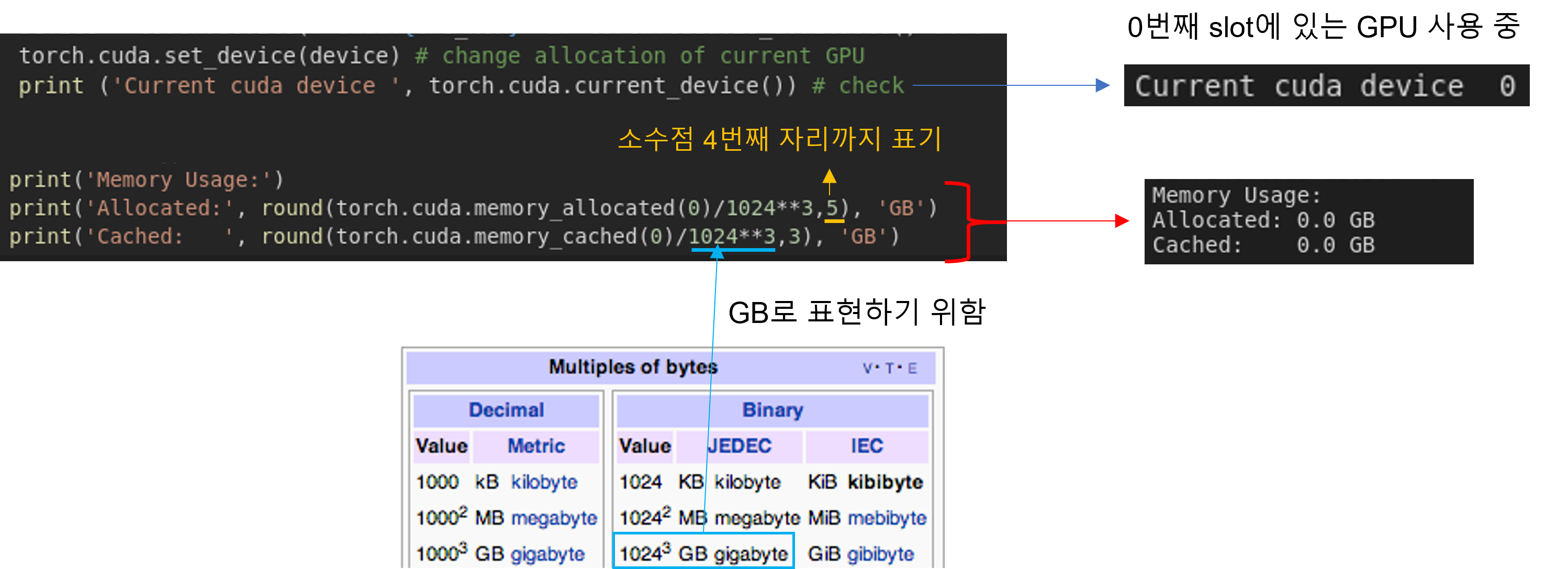
아래와 같이 코드를 수행해도 GPU 상의 메모리를 확인할 수 있는데, 아래 코드를 이용하면 아무런 메모리도 올라가 있지 않다는걸 확인할 수 있습니다. torch 관련한 코드로 GPU 메모리를 확인하면 torch 코드로 GPU 상에 데이터를 업로드 하지 않은 이상 GPU 메모리 용량이 0으로 표현되는듯 합니다.

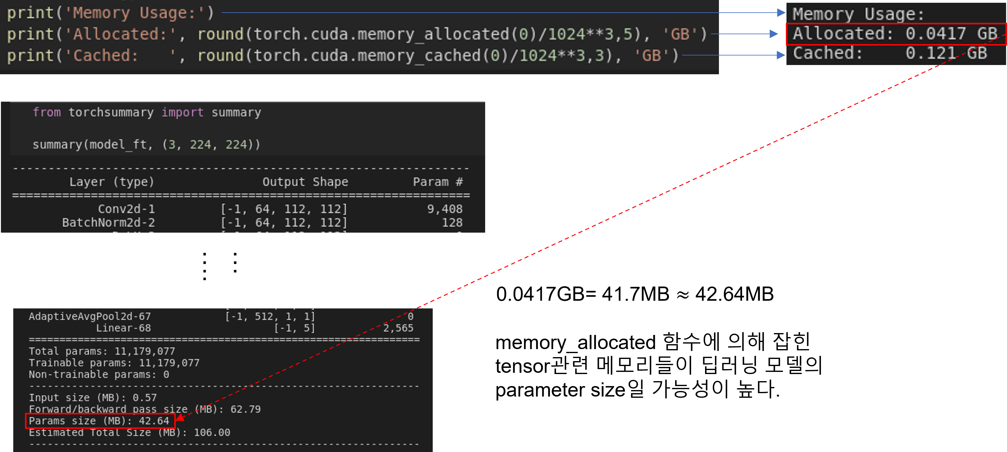
이번엔 아래 코드를 수행하여 딥러닝 모델을 GPU에 업로드 하고, GPU 메모리를 확인해 보도록 하겠습니다.

• model.to(device): When loading a model on a GPU that was trained and saved on GPU, simply convert the initialized model to a CUDA optimized model using model.to(torch.device('cuda')).

• torch.cuda.memory_allocated 설명
  • You can use memory_allocated() and max_memory_allocated() to monitor memory occupied by tensors, and use memory_reserved() and max_memory_reserved() to monitor the total amount of memory managed by the caching allocator.
• torch.cuda.memory_cached 설명
  • PyTorch uses a caching memory allocator to speed up memory allocations.
  • This allows fast memory deallocation without device synchronizations.

• However, the unused memory managed by the allocator will still show as if used in nvidia-smi.
  
  • The nvidia-smi number includes space the allocated by the CUDA driver when it loads PyTorch.
  • This can be quite large because PyTorch includes many CUDA kernels. On a P100, I’ve seen an overhead of ~487 MB.
  • This memory isn’t reported by the torch.cuda.xxx_memory functions because it’s not allocated by the program and there isn’t a good way to measure it outside of looking at nvidia-smi.
  • Our tensor is too small. The caching allocator allocates memory with a minimum size and a block size so it may allocate a bit more memory than the number of elements in your tensors.
  • Things like cuda ctx, cuda rng state, cudnn ctx, cufft plans, and other gpu memory your other libraries may use are not counted in the torch.cuda.* stats.

지금까지 배운 내용(1.Data load(Feat. CUDA), 2.Data Preprocessing(Feat. Augmentation))을 코드로 요약 하면 아래와 같습니다.

# License: BSD
# Author: Sasank Chilamkurthy

from __future__ import print_function, division

import torch
import torch.nn as nn
import torch.optim as optim
from torch.optim import lr_scheduler
import numpy as np
import torchvision
from torchvision import datasets, models, transforms
import matplotlib.pyplot as plt
import time
import os
import copy

plt.ion()   # interactive mode

# Data augmentation and normalization for training
# Just normalization for validation
data_transforms = {
    'train': transforms.Compose([
        transforms.RandomResizedCrop(224),
        transforms.RandomHorizontalFlip(),
        transforms.ToTensor(),
        transforms.Normalize([0.485, 0.456, 0.406], [0.229, 0.224, 0.225])
    ]),
    'val': transforms.Compose([
        transforms.Resize(256),
        transforms.CenterCrop(224),
        transforms.ToTensor(),
        transforms.Normalize([0.485, 0.456, 0.406], [0.229, 0.224, 0.225])
    ]),
}

data_dir = 'data/hymenoptera_data'
image_datasets = {x: datasets.ImageFolder(os.path.join(data_dir, x),
                                          data_transforms[x])
                  for x in ['train', 'val']}
dataloaders = {x: torch.utils.data.DataLoader(image_datasets[x], batch_size=4,
                                             shuffle=True, num_workers=4)
              for x in ['train', 'val']}
dataset_sizes = {x: len(image_datasets[x]) for x in ['train', 'val']}
class_names = image_datasets['train'].classes

device = torch.device("cuda:0" if torch.cuda.is_available() else "cpu")

def imshow(inp, title=None):
    """Imshow for Tensor."""
    inp = inp.numpy().transpose((1, 2, 0))
    mean = np.array([0.485, 0.456, 0.406])
    std = np.array([0.229, 0.224, 0.225])
    inp = std * inp + mean
    inp = np.clip(inp, 0, 1)
    plt.imshow(inp)
    if title is not None:
        plt.title(title)
    plt.pause(0.001)  # pause a bit so that plots are updated


# Get a batch of training data
inputs, classes = next(iter(dataloaders['train']))

# Make a grid from batch
out = torchvision.utils.make_grid(inputs)

imshow(out, title=[class_names[x] for x in classes])

model_ft = models.resnet18(pretrained=True)
num_ftrs = model_ft.fc.in_features
# Here the size of each output sample is set to 2.
# Alternatively, it can be generalized to nn.Linear(num_ftrs, len(class_names)).
model_ft.fc = nn.Linear(num_ftrs, 2)

model_ft = model_ft.to(device)

다음 글에서는 딥러닝 모델이 학습할 방향성을 결정해주는 loss function, optimizer, learning rate schedule 에 대해서 알아보도록 하겠습니다.

(↓↓↓ 다음 글에서 배울 코드내용↓↓↓)

criterion = nn.CrossEntropyLoss()

# Observe that all parameters are being optimized
optimizer_ft = optim.SGD(model_ft.parameters(), lr=0.001, momentum=0.9)

# Decay LR by a factor of 0.1 every 7 epochs
exp_lr_scheduler = lr_scheduler.StepLR(optimizer_ft, step_size=7, gamma=0.1)

안녕하세요.

이번 글에서는 pytorch를 이용해서 대표적인 CNN 모델인 ResNet을 implementation 하는데 필요한 코드를 line by line으로 설명해보려고 합니다.

ResNet을 구현할 줄 아시면 전통적인 CNN 모델들은 자유롭게 구현하는데 어려움이 없을거라 생각됩니다. 

우선 pytorch에서 resnet 모델을 불러오는 코드는 아래 한 줄로 가능합니다.

model = resnet50().to(device)

그렇다면 resnet50() 이라는 함수가 어떤 과정을 통해 실행되는지 살펴봐야겠죠?

지금부터 이 과정을 순차대로 살펴보도록 하겠습니다.

※ 최종코드는 제일 아래에 있으니 참고해주세요!

※ 대부분 PPT 슬라이드에 설명한 내용을 이미지로 만들어 업로드했기 때문에 글씨가 잘 안보일 수도 있습니다. 그래서 PPT파일을 따로 첨부 하도록 하겠습니다.

0. ResNet() 함수 호출

• 먼저 resnet50()을 호출하면 ResNet(BottleNeck, [3,4,6,3]) 함수를 호출하게됩니다.
• ResNet 함수 내부를 대략적으로 살펴보면 ResNet50 구조를 파악할 수 있습니다.

1. (BottleNeck 적용 전) 첫 번째 conv layer

• ResNet 함수에서 첫 번째 conv layer 부터 살펴보도록 하겠습니다.

2. 두 번째 Conv layer

• 두 번째 Conv layer 부터 bottleneck이 적용됩니다. 앞서 노란색 영역인 첫 번째 conv layer를 지나면, 아래 빨간색 영역의 첫 번째 bottleneck 연산이 진행됩니다.
• 우선 첫 번째 bottleneck을 간단히 도식화하면 아래와 같이 나타낼 수 있습니다.

• Bottleneck이 포함된 conv layer를 생성하기 위해 make_layer 함수가 실행되야 하는데, make_layer 함수에 작성된 python 기본 문법들을 먼저 설명하겠습니다. 
  • 연산자를 이용한 리스트 생성
  • for in 반복문 (with 리스트)
  • 리스트 인자 함수
  • Sequential 함수

• sequential 함수 설명

2-1. 두 번째 Conv layer에서 첫 번째 BottleNeck 적용 (make_layer(), BottleNeck()=block() 함수 호출)

2-2. 두 번째 Conv layer에서 두 번째 BottleNeck 적용 (make_layer(), BottleNeck()=block() 함수 호출)

2-3. 두 번째 Conv layer에서 세 번째 BottleNeck 적용 (make_layer(), BottleNeck()=block() 함수 호출)

3. 세 번째 Conv layer

3-1. 세 번째 Conv layer에서 첫 번째 BottleNeck 적용 (make_layer(), BottleNeck()=block() 함수 호출 + Down_sampling)

• 여기서 부터는 첫 번째 bottleNeck에 shortcut (for skip connection) 적용을 위해 down_sampling이 된다는 점을 알아두시면 좋을 것 같습니다.
• Down_sampling은 conv filter의 stride를 2로 설정함으로써 진행이 됩니다.

3-2. 세 번째 Conv layer에서 두 번째 BottleNeck 적용 (make_layer(), BottleNeck()=block() 함수 호출)

3-3. 세 번째 Conv layer에서 세 번째 BottleNeck 적용 (make_layer(), BottleNeck()=block() 함수 호출)

• block 함수 부분은 이전과 설명이 동일 하므로 이제부터는 생략하겠습니다.

3-4. 세 번째 Conv layer에서 세 번째 BottleNeck 적용 (make_layer(), BottleNeck()=block() 함수 호출)

4, 5. 네 번째 Conv layer, 다섯 번째 Conv layer

• 여기서부터는 위에서 설명한 내용의 반복이라 make_layer, block 함수 실행과정은 생략하도록 하겠습니다.

6. Average pooling, FC layer, Softmax

7. Weight initialization

(↓↓↓ 가중치 초기화 관련 API ↓↓↓)

https://pytorch.org/docs/stable/nn.init.html

8. Model Show

• 앞서 작성한 코드가 올바로 작성됐는지 해당 모델 구조를 들여다보는 세 가지 방법에 대해서 알아보겠습니다.

8-1. model.modules()

8-2. model.named_parameters()

8-3. summary()

9. 최종 코드

# model
import torch
import torch.nn as nn
import torch.nn.functional as F
from torchsummary import summary

class ResNet(nn.Module):
    def __init__(self, block, num_block, num_classes=10, init_weights=True):
        super().__init__()

        self.in_channels=64

        self.conv1 = nn.Sequential(
            nn.Conv2d(3, 64, kernel_size=7, stride=2, padding=3, bias=False),
            nn.BatchNorm2d(64),
            nn.ReLU(),
            nn.MaxPool2d(kernel_size=3, stride=2, padding=1)
        )

        self.conv2_x = self._make_layer(block, 64, num_block[0], 1)
        self.conv3_x = self._make_layer(block, 128, num_block[1], 2)
        self.conv4_x = self._make_layer(block, 256, num_block[2], 2)
        self.conv5_x = self._make_layer(block, 512, num_block[3], 2)

        self.avg_pool = nn.AdaptiveAvgPool2d((1,1))
        self.fc = nn.Linear(512 * block.expansion, num_classes)

        # weights inittialization
        if init_weights:
            self._initialize_weights()

    def _make_layer(self, block, out_channels, num_blocks, stride):
        strides = [stride] + [1] * (num_blocks - 1)
        layers = []
        ith_block = 1
        for stride in strides:
            layers.append(block(self.in_channels, out_channels, stride, ith_block))
            self.in_channels = out_channels * block.expansion
            ith_block = ith_block+1

        return nn.Sequential(*layers)

    def forward(self,x):
        output = self.conv1(x)
        output = self.conv2_x(output)
        x = self.conv3_x(output)
        x = self.conv4_x(x)
        x = self.conv5_x(x)
        x = self.avg_pool(x)
        x = x.view(x.size(0), -1)
        x = self.fc(x)
        return x

    # define weight initialization function
    def _initialize_weights(self):
        for m in self.modules():
            if isinstance(m, nn.Conv2d):
                nn.init.kaiming_normal_(m.weight, mode='fan_out', nonlinearity='relu')
                if m.bias is not None:
                    nn.init.constant_(m.bias, 0)
            elif isinstance(m, nn.BatchNorm2d):
                nn.init.constant_(m.weight, 1)
                nn.init.constant_(m.bias, 0)
            elif isinstance(m, nn.Linear):
                nn.init.normal_(m.weight, 0, 0.01)
                nn.init.constant_(m.bias, 0)


def resnet50():
    return ResNet(BottleNeck, [3,4,6,3])

class BottleNeck(nn.Module):
    expansion = 4
    def __init__(self, in_channels, out_channels, stride=1, ith_block=1):
        super().__init__()

        self.residual_function = nn.Sequential(
            nn.Conv2d(in_channels, out_channels, kernel_size=1, stride=1, bias=False),
            nn.BatchNorm2d(out_channels),
            nn.ReLU(),
            nn.Conv2d(out_channels, out_channels, kernel_size=3, stride=stride, padding=1, bias=False),
            nn.BatchNorm2d(out_channels),
            nn.ReLU(),
            nn.Conv2d(out_channels, out_channels * BottleNeck.expansion, kernel_size=1, stride=1, bias=False),
            nn.BatchNorm2d(out_channels * BottleNeck.expansion),
        )

        self.shortcut = nn.Sequential()

        if stride == 1 and ith_block == 1: #첫 번째 block에서의 shortcut (or identity) 을 적용해주기 위해서는 channel 조정필요
            self.shortcut = nn.Sequential(nn.Conv2d(in_channels, out_channels * BottleNeck.expansion, kernel_size=1, stride=1), 
                                          nn.BatchNorm2d(out_channels*BottleNeck.expansion))

        if stride != 1 or in_channels != out_channels * BottleNeck.expansion: #feature size_downsampling
            self.shortcut = nn.Sequential(
                nn.Conv2d(in_channels, out_channels*BottleNeck.expansion, kernel_size=1, stride=stride, bias=False),
                nn.BatchNorm2d(out_channels*BottleNeck.expansion)
            )
            

        self.relu = nn.ReLU() 

    def forward(self, x):
        x = self.residual_function(x) + self.shortcut(x)
        x = self.relu(x)
        return x

device = torch.device('cuda' if torch.cuda.is_available() else 'cpu')
model = resnet50().to(device)
x = torch.randn(3, 3, 224, 224).to(device)
output = model(x)
print(output.size())

for name, param in model.named_parameters():
    print(name, param.size())

for m in model.modules():
    print(m)

#ResNet50 모델 summary 
summary(model, (3, 224, 224), device=device.type)

지금까지 ResNet50을 pytorch로 구현한 code에 대해서 설명해봤습니다.

다음 글에서는 Pretrained model를 불러드려와 transfer learning을 적용시키는 코드에 대해 설명하도록 하겠습니다.